

TimeSeriesAggregate
TimeSeriesAggregate[tes,dt]
computes the mean value of time or event series tes over non-overlapping windows of width dt.
TimeSeriesAggregate[tes,dt,f]
applies the function f to the values of tes in non-overlapping windows of width dt.
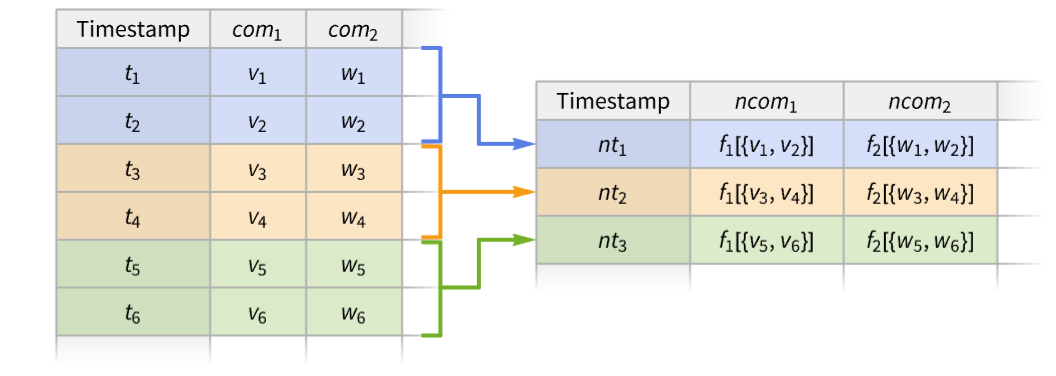
TimeSeriesAggregate[tes,dt,{ncom1f1,ncom2f2,…}]
constructs a new series with components ncomi for functions fi.
Details
- TimeSeriesAggregate is typically used in time and event series analysis to compute aggregated statistics like yearly averages or monthly totals.
- TimeSeriesAggregate breaks the series tes into disjoint left-closed and right-open windows of equal width dt and applies a function f to the values in each window.
- Possible forms of time or event series data tes include:
-
TimeSeries[…] continuous time-ordered sampled data EventSeries[…] collection of temporal events with values TemporalData[…] one or more paths composed of time-value pairs {{t1,x1},{t2,x2},…} list of time-value pairs {x1,x2,…} list of values with implied integer times starting at 0 - If there are no values in a window, the window is ignored.
- The window width dt can be given as a positive number, a Quantity, or as a date increment.
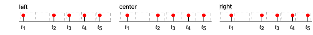
- The window width specification dt can be extended to {dt,align}, specifying also the alignment of new timestamps within each window.
- Settings for window alignment align include Left, Center (default), and Right.
- A component "com" in a time or event series tes can be used as an argument to the aggregation function f using the syntax f[…,#com,…]&.
- For a simple time series with no named components, values can be accessed using either f[…,#,…]& or f[…,#Value,…]&.
- TimeSeriesAggregate threads pathwise for TemporalData objects with multiple paths.
Examples
open all close allBasic Examples (3)
Average successive pairs of values in a time series:
TimeSeries[{Subscript[x, 1], Subscript[x, 2], Subscript[x, 3], Subscript[x, 4], Subscript[x, 5], Subscript[x, 6]}, {1}]TimeSeriesAggregate[%, 2]Normal[%]Add successive pairs of value in a list:
TimeSeriesAggregate[{Subscript[x, 1], Subscript[x, 2], Subscript[x, 3], Subscript[x, 4], Subscript[x, 5], Subscript[x, 6]}, 2, Total]Specify the value components to use as function arguments in a multicomponent time series:
ts = TimeSeries[{{11, "cat"}, {17, "dog"}, {13, "fox"}, {14, "cow"}, {10, "owl"}}, {0.}, {"a", "b"}];
Tabular[ts]TimeSeriesAggregate[ts, 3, {"max" -> (Max[#a]&), "joined" -> (StringJoin[#b]&)}]Tabular[%]Scope (22)
Basic Uses (5)
Map a function f over data with blocks of width 2:
data = TimeSeries[{Subscript[x, 1], Subscript[x, 2], Subscript[x, 3], Subscript[x, 4], Subscript[x, 5]}, {1}]TimeSeriesAggregate[data, 2, f]%//NormalCompute the 95![]() quantile for windows of width 0.05:
quantile for windows of width 0.05:
data = RandomFunction[WienerProcess[], {0, 1, .01}]TimeSeriesAggregate[data, 0.05, Quantile[#, 95 / 100]&]ListLinePlot[{data, %}]Find a quartile envelope for blocks of size 10:
data = TimeSeries[Accumulate@RandomReal[{-1, 1}, 250]]TimeSeriesAggregate[data, 10, Quartiles]Show[ListLinePlot[%], ListPlot[data, PlotStyle -> Gray]]Compute the quarterly standard deviation for a financial time series:
data = FinancialData["GOOGL", {DateObject[{2019, 1, 1}, "Day"], DateObject[{2026, 1, 31}, "Day"]}]TimeSeriesAggregate[data, "Quarter", StandardDeviation]DateListPlot[%, GridLines -> {True, None}, PlotRange -> All]Aggregate multiple paths simultaneously:
data = RandomFunction[BrownianBridgeProcess[{0, -1}, {2, 1}], {0, 2, .01}, 3]TimeSeriesAggregate[data, .15]Show[ListPlot[data], ListLinePlot[%, PlotStyle -> Thick]]Data Types (8)
Aggregate a vector in blocks of 4 using a function f:
v = RandomInteger[{-10, 10}, 10]TimeSeriesAggregate[v, 4, f]Find the two-year average for a list of time-value pairs:
data = {{"2005", 1}, {"2006", -1}, {"2007", 3}, {"2008", 6}, {"2009", -2}, {"2010", 4}, {"2011", 5}, {"2012", 4}, {"2013", 6}};TimeSeriesAggregate[data, {2, "Year"}]DateListPlot[{data, %}, PlotTheme -> "Detailed"]Compute the maximum for width-10 segments of a TimeSeries:
ts = TimeSeries[TimeEventSeries`TimestampData[Association["UniformlySpacedQ" -> True, "Count" -> 100,
   "Endpoints" -> TabularColumn[Association["Data" -> {{0, 99}, {}, None},
      "ElementType" -> "Integer64"]], "MinimumTimeIncrement" -> 1, "Caller ...  -5.83329995009813, -5.365194518466113, -5.614668108914484,
      -6.477246191853266, -7.461704439607946, -6.79657593242878, -5.864937981765857,
-6.27785271209235, -5.841962111797332}, {}, None}, "ElementType" -> "Real64"]], Association[]];TimeSeriesAggregate[ts, 10, Max]ListLinePlot[{ts, %}]Compute a width-10 median for TemporalData:
td = TemporalData[Automatic, {{{0.4948076687033609, -0.49167253739690864, -1.1692407506834863,
    -0.25256398166927063, -1.0324595217335713, -1.5365451139092143, -2.0662926057486564,
    -1.7443987109156156, -2.6969884040577115, -3.663349952028885, - ... 13,
    -5.365194518466113, -5.614668108914484, -6.477246191853266, -7.461704439607946,
    -6.79657593242878, -5.864937981765857, -6.27785271209235, -5.841962111797332}}, {{0, 99, 1}},
1, {"Discrete", 1}, {"Discrete", 1}, 1, {}}, False, 10.];TimeSeriesAggregate[td, 10, Median]ListLinePlot[{td, %}]Compute a width-5 total for an EventSeries:
es = EventSeries[TimeEventSeries`TimestampData[Association["UniformlySpacedQ" -> True, "Count" -> 100,
   "Endpoints" -> TabularColumn[Association["Data" -> {{0, 99}, {}, None},
      "ElementType" -> "Integer64"]], "MinimumTimeIncrement" -> 1, "Calle ... 1, 1, 0, 1, 1, 0, 0, 0,
      0, 0, 0, 0, 0, 1, 0, 0, 0, 1, 1, 1, 0, 0, 0, 0, 0, 0, 1, 1, 0, 1, 0, 0, 1, 0, 1, 0, 1, 1, 1,
      0, 0, 1, 1, 1, 0, 0, 1, 1, 1, 1, 1, 0, 0, 0, 1, 1, 0}, {}, None},
"ElementType" -> "Integer64"]], Association[]];TimeSeriesAggregate[es, 5, Total]Show[ListLinePlot[%, InterpolationOrder -> 0], ListPlot[es, PlotStyle -> {Gray, AbsolutePointSize[3]}]]Compute a six-month variance for multiple paths simultaneously:
td = TemporalData[«4»];TimeSeriesAggregate[td, {6, "Month"}, Variance]DateListPlot[%, GridLines -> {Automatic, None}, PlotRange -> All, PlotLegends -> {"HP", "IBM"}]Aggregate over vector-valued data:
α = {{.2, .1}, {-.3, .2}};
β = {{.2, .5}, {-.2, .6}};
Σ = {{1, 0}, {0, .3}};
arima = RandomFunction[SARIMAProcess[{α}, 1, {}, {6, {β}, 1, {}}, Σ], {1, 10 ^ 3}]//TimeSeriesres = TimeSeriesAggregate[arima, 5, Map[Max[#] - Min[#]&, Transpose[#]]&]ListPointPlot3D[Table[Join[{t}, Normal[res[t]]], {t, 4, 998}], BoxRatios -> 1, ColorFunction -> Function[{t, x, y}, (ColorData["BlueGreenYellow"][t])], AxesLabel -> {"t", "x", "y"}]Aggregate over a time series involving quantities:
ts = TimeSeries[Quantity[{0, 16, 9, 3, 7, 2, 17, 10, 6, 12}, "Meters"]]TimeSeriesAggregate[ts, 2]ListLinePlot[{ts, %}, PlotLegends -> {"original time series", "aggregated time series"}, Filling -> Axis, AxesLabel -> Automatic]Window Widths (5)
data = TimeSeries[{Subscript[x, 1], Subscript[x, 2], Subscript[x, 3], Subscript[x, 4]}, {1}]TimeSeriesAggregate[data, 2, f]//NormalTimeSeriesAggregate[data, {2, Center}, f]//NormalAverage over windows spanning 14 days:
data = FinancialData["APP", "2024"]TimeSeriesAggregate[data, Quantity[14, "Days"]];DateListPlot[{data, %}, GridLines -> {Automatic, None}]Average over windows spanning the Quantity of two quarters:
data = FinancialData["GE", "2010"]TimeSeriesAggregate[data, Quantity[2, "QuarterYears"]]DateListPlot[{data, %}, GridLines -> {Automatic, None}]Average over windows spanning three weeks and two days:
data = FinancialData["SBUX", "2020"]w = {{3, "Week"}, {2, "Day"}};TimeSeriesAggregate[data, w]DateListPlot[{data, %}, GridLines -> {Automatic, None}]data = FinancialData["SP500", "2020"]avg[w_] := TimeSeriesAggregate[data, w]Moving averages with increasing window width:
wspec = {{1, "Week"}, {1, "Month"}, {1, "Quarter"}};Map[DateListPlot[avg[#], PlotLabel -> Last[#], ...]&, wspec]Alignment (4)
Align new times with the center of the windows:
data = TimeSeries[{Subscript[x, 1], Subscript[x, 2], Subscript[x, 3], Subscript[x, 4], Subscript[x, 5], Subscript[x, 6], Subscript[x, 7]}, {1}]TimeSeriesAggregate[data, {3, Center}, f]//NormalCenter alignment is used by default:
TimeSeriesAggregate[data, 3, f]//NormalAlign new times with the right side of the windows:
data = TimeSeries[{Subscript[x, 1], Subscript[x, 2], Subscript[x, 3], Subscript[x, 4], Subscript[x, 5], Subscript[x, 6], Subscript[x, 7]}, {1}]TimeSeriesAggregate[data, {3, Right}, f]//NormalAlign new times with the left side of the windows:
data = TimeSeries[{Subscript[x, 1], Subscript[x, 2], Subscript[x, 3], Subscript[x, 4], Subscript[x, 5], Subscript[x, 6], Subscript[x, 7]}, {1}]TimeSeriesAggregate[data, {3, Left}, f]//Normaldata = TimeSeries[Accumulate[RandomReal[{-1, 1}, 100]]]mavg = Table[TimeSeriesAggregate[data, {10, align}], {align, {Right, Center, Left}}];The values are all equivalent:
Equal@@(#["Values"]& /@ mavg)Equal@@(#["Times"]& /@ mavg)Show[ListPlot[data, PlotStyle -> Gray], ListLinePlot[mavg, PlotStyle -> Thick, PlotLegends -> {Right, Center, Left}]]Applications (3)
Departures (1)
Take an event series of flight departures from an airport:
times = EntityValue[FlightData[Entity["Airport", "KORD"] -> All, "Flights", DateObject[{2022, 11, 11}]], "DepartureTime"];departures = EventSeries[1, {times}, TimeZone -> "America/Chicago"]Aggregate departures per hour:
res = TimeSeriesAggregate[departures, Quantity[1, "Hours"], Total]Show[DateHistogram[departures["Timestamps"], Quantity[1, "Hours"]], ListLinePlot[res]]Labor Force (1)
Visualize the growth of labor force in California based on monthly data:
CAMonthlyLaborForce = EntityValue[...]growth = TimeSeriesAggregate[CAMonthlyLaborForce, {1, "Year"}]DateListPlot[growth, GridLines -> True, FrameLabel -> Automatic, PlotLabel -> "Annual average labor force in California"]Market Volatility (1)
Identify periods of high volatility in the S&P 500:
data = FinancialData["SP500", All]smooth = TimeSeriesAggregate[data, Quantity[5, "Years"], StandardDeviation];DateListPlot[smooth, PlotRange -> All, PlotTheme -> "Business"]smooth = TimeSeriesAggregate[data, Quantity[1, "Years"], InterquartileRange];DateListPlot[smooth, PlotRange -> All, PlotTheme -> "Business"]smooth = TimeSeriesAggregate[data, Quantity[2, "Years"], Max[#] - Min[#]&];DateListPlot[smooth, PlotRange -> All, PlotTheme -> "Business"]Properties & Relations (1)
Independently of the alignment, the windows are closed on the left and open on the right:
data = TimeSeries[{{0, a}, {1, b}, {2, c}}]left = TimeSeriesAggregate[data, {2, Left}, Total];
left//NormalIt is possible that more timestamps need to be added:
center = TimeSeriesAggregate[data, {2, Center}, Total];
center//Normalright = TimeSeriesAggregate[data, {2, Right}, Total];
right//NormalText
Wolfram Research (2014), TimeSeriesAggregate, Wolfram Language function, https://reference.wolfram.com/language/ref/TimeSeriesAggregate.html (updated 2026).
CMS
Wolfram Language. 2014. "TimeSeriesAggregate." Wolfram Language & System Documentation Center. Wolfram Research. Last Modified 2026. https://reference.wolfram.com/language/ref/TimeSeriesAggregate.html.
APA
Wolfram Language. (2014). TimeSeriesAggregate. Wolfram Language & System Documentation Center. Retrieved from https://reference.wolfram.com/language/ref/TimeSeriesAggregate.html