


MovingMap
MovingMap[f,tes,wspec]
applies f to windows specified by wspec in the time or event series data tes.
MovingMap[f,tes,wspec,padding]
pads tes using padding.
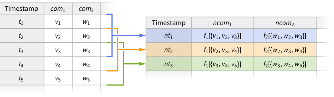
MovingMap[{ncomp1f1,ncomp2f2,…},tes,…]
constructs a new time series with components ncompi obtained by applying the functions fi to windows of tes.
Details
- MovingMap is also known as rolling or sliding map.
- MovingMap is typically used to smooth the time series data by applying a function to the list of values in each of the time windows.
- Possible forms of time series data tes include:
-
TimeSeries[…] continuous time-ordered sampled data EventSeries[…] collection of temporal events with values TemporalData[…] one or more paths composed of time-value pairs {{t1,x1},{t2,x2},…} list of time-value pairs {x1,x2,…} list of values with implied integer times starting at 0 - A function f of a single argument gets applied to a list of values {xi,xi+1,…} for each window. »
- A pure function f can access values, times, boundary values and boundary times for each window using the following arguments: »
-
#Values or #1 data values within the window #Times or #2 data times within the window #BoundaryValues or #3 resampled values at window boundaries #BoundaryTimes or #4 times at window boundaries #Dates or #5 data dates within the window - By default, f is expected to compute a single value for each window and the time is computed automatically. Using a function f that gives output as rules {τi,…}{vi,…} allows control over both time and value as well as producing multiple values per window. »
- Possible window specifications wspec include:
-
size, {size} specify size, with Automatic alignment and positions {size,align} specify size and alignment, with Automatic positions {size,align,wpos} specify size, alignment and positions » - Window size can be given as the following:
-
w positive number, taken to mean days Quantity[w,timeunit] duration w in units of timeunit Quantity[n,"Events"] events count n defines the window size - The window size may be varying in an absolute sense when referring to relative units such as "Month" or "Events".
- Window placements {τ1,…,τm} are specified by wpos. With timestamps {t1,…,tn}, wpos can be one of the following:
-
Automatic use tes timestamps τi=ti {τmin,τmax} use τi=tk+i such that τmin≤tk+i≤τmax {Automatic,τmax} equivalent to {t1,τmax} {τmin,Automatic} equivalent to {τmin,tn} {τmin,τmax,dτ} use τ1=τmin, τ2=τmin+dτ, etc. {{τ1,…,τm}} use explicit τ1, τ2, etc. - By default, the timestamps of the output are the window placements {τ1,…,τm}.
- Window alignment align determines relative position of τi within the window. The possible settings include Right (default), Left and Center.
- Settings for padding include:
-
Automatic only keep non-overhanging windows (default) None no padding, keep all windows valuepadding equivalent to {Automatic,valuepadding} {timepadding,valuepadding} padding settings for times and values - Settings for valuepadding can be any valid specification recognized by ArrayPad.
- Settings for timepadding include:
-
Automatic pad uniformly median time-step size Δt pad uniformly with step-size Δt {Δt1,Δt2,…} cyclically pad with steps Δti "ReflectedDifferences" reflections of the differences between times "PeriodicDifferences" cyclically pad with steps ti+1-ti - MovingMap threads pathwise for TemporalData objects with multiple paths.


Examples
open all close allBasic Examples (4)
Compute moving average over a window of width 2:
MovingMap[Mean, TimeSeries[{Subscript[x, 1], Subscript[x, 2], Subscript[x, 3], Subscript[x, 4], Subscript[x, 5]}], 2]For a uniformly spaced time series, each window produces the mean of three elements:
Normal[%]Compute moving mean of an irregularly spaced time series:
ts = TimeSeries[{Subscript[x, 1], Subscript[x, 2], Subscript[x, 3], Subscript[x, 4], Subscript[x, 5], Subscript[x, 6], Subscript[x, 7]}, {Prime[Range[7]]}]Normal[ts]MovingMap[Mean, ts, 3]For an irregularly spaced time series, the number of elements per window can vary:
Normal[%]Take a time series of stock prices in US dollars at open and close:
ts = TimeSeries[TimeEventSeries`TimestampData[Association["UniformlySpacedQ" -> False,
   "Timestamps" -> TabularColumn[Association[
      "Data" -> {502, {{{1704153600000, 1704240000000, 1704326400000, 1704412800000, 1704672000000,
           1704758 ... 0999755859375,
                273.3999938964844, 273.760009765625, 273.0799865722656, 271.8599853515625}, {
                }, None}}, None}, "ElementType" -> TypeSpecifier["Quantity"]["Real64",
"USDollars"]]]}}]]]], Association[]];ColumnTypes[ts]Compute the moving mean of the price at close:
MovingMap[Mean[#close]&, ts, {Quantity[3, "Months"], Center}]Visualize the moving mean with the original data:
Show[DateListLogPlot[ts -> "close", PlotStyle -> GrayLevel[.7]], DateListLogPlot[%, Joined -> True, PlotStyle -> Thick]]Compute simultaneously moving min and moving max of a time series over the same windows:
ts = TimeSeries[Accumulate[RandomReal[{-1, 1}, 50]]]MovingMap[{"min" -> (Min[#Values]&), "max" -> (Max[#Values]&)}, ts, {5, Center}]Visualize the components and the original data:
ListLinePlot[{ts, % -> "min", % -> "max"}]Scope (35)
Basic Uses (7)
Map a function f over data with a window of width two units of time:
data = {{1, Subscript[x, 1]}, {2, Subscript[x, 2]}, {4, Subscript[x, 4]}, {6, Subscript[x, 6]}, {7, Subscript[x, 7]}, {12, Subscript[x, 12]}};MovingMap[f, data, 2]Map a function f over data with a three-events window:
MovingMap[f, data, Quantity[3, "Events"]]Take a time series with two value components:
ts = TimeSeries[TimeEventSeries`TimestampData[Association["UniformlySpacedQ" -> True, "Count" -> 6,
   "Endpoints" -> TabularColumn[Association["Data" -> {{0, 0}, {}, DataStructure["BitVector",
         {"Data" -> ByteArray["/Q=="], "Capacity" -> 2, " ... ne}, "ElementType" ->
            "String"]]}}]]]], Association["ResamplingMethod" ->
   Association["c1" -> {"Interpolation", InterpolationOrder -> 1}, "c2" -> "PreviousElement"],
"TimeWindow" -> Interval[{0, 5}], "MetaInformation" -> None]];Normal[ts]Compute a moving map of the consecutive character concatenations:
MovingMap[StringJoin[#c2]&, ts, 2]Normal[%]Compute a moving quantile for some data:
data = RandomFunction[WienerProcess[], {0, 10, 0.1}]Use centered window of unit size:
mq = MovingMap[Quantile[#, 0.75]&, data, {1, Center}]ListLinePlot[{data, mq}]Find a moving quartile envelope:
data = TimeSeries[Accumulate[RandomReal[{-1, 1}, 250]], {1}]q = MovingMap[Quartiles, data, {12, Center}]ListLinePlot[q]Smooth an irregularly spaced time series:
data = TimeSeries[FinancialData["SBUX", {"2020", "2025"}]]RegularlySampledQ[data]MovingMap[Median, data, Quantity[3, "Months"]]Show[DateListLogPlot[data, PlotStyle -> GrayLevel[.7]], DateListLogPlot[%, Joined -> True, PlotStyle -> Thick]]Find a yearly moving average of SP500 time series:
ts = FinancialData["SP500", {"2020", "2025"}]MovingMap[Mean, ts, "Year"]Find a yearly moving average of the time series, placing windows monthly:
MovingMap[Mean, ts, {"Year", Right, "Month"}]Place windows monthly at the first day of each month and use reflected value padding:
MovingMap[Mean, ts, {"Year", Right, {"Jan 1 2020", Automatic, "Month"}}, "Reflected"]DateListPlot[{ts, %}, Joined -> {False, True}, PlotStyle -> {PointSize[Tiny], Automatic, Automatic}]Smooth multiple paths simultaneously:
data = RandomFunction[BrownianBridgeProcess[{0, -1}, {2, 1}], {0, 2, .01}, 3]Use a centered window and reflected padding:
avg = MovingMap[Mean, data, {0.1, Center}, "Reflected"]Show[ListPlot[data], ListLinePlot[avg]]Data Types (7)
Create a generic moving function for a vector:
v = Table[Subscript[x, t], {t, 1, 12}]MovingMap[f, v, 2]Compute a moving average for a list of time-value pairs:
data = {{"2005", 1}, {"2006", -1}, {"2007", 3}, {"2008", 6}, {"2009", -2}, {"2010", 4}, {"2011", 5}, {"2012", 4}, {"2013", 6}, {"2014", 3}};mavg = MovingMap[Mean, data, "Year"];DateListPlot[{data, mavg}, Joined -> True]Compute a moving GeometricMean for a TimeSeries:
ts = TimeSeries[TimeEventSeries`TimestampData[Association["UniformlySpacedQ" -> True, "Count" -> 64,
   "Endpoints" -> TabularColumn[Association["Data" -> {{1, 64}, {}, None},
      "ElementType" -> "Integer64"]], "MinimumTimeIncrement" -> 1, "Caller" ... 87661, 0.2380279869779624, 0.18426497446026752,
      0.13307598834536247, 0.09329283514730177}, {}, None}, "ElementType" -> "Real64"]],
 Association["ResamplingMethod" -> "LinearInterpolation", "TimeObservationWindow" ->
Interval[{1, 64}]]];MovingMap[GeometricMean, ts, 5, None]ListLinePlot[{ts, %}]Compute a moving median for a TemporalData:
td = RandomFunction[ARMAProcess[{5 / 6}, {1 / 2}, 1], {0, 100}]MovingMap[Median, td, 10, None]ListLinePlot[{td, %}]Compute a moving total for an EventSeries:
es = EventSeries[TimeEventSeries`TimestampData[Association["UniformlySpacedQ" -> True, "Count" -> 100,
   "Endpoints" -> TabularColumn[Association["Data" -> {{0, 99}, {}, None},
      "ElementType" -> "Integer64"]], "MinimumTimeIncrement" -> 1, "Calle ... , 1, 0, 0, 0, 1, 1, 1, 0, 0, 0, 0, 0, 0, 1, 1, 0, 1, 0, 0, 1, 0, 1, 0, 1, 1, 1,
      0, 0, 1, 1, 1, 0, 0, 1, 1, 1, 1, 1, 0, 0, 0, 1, 1, 0}, {}, None},
"ElementType" -> "Integer64"]], Association["TimeObservationWindow" -> Interval[{0, 99}]]];MovingMap[Total, es, 10]ListPlot[{%, es}, Filling -> 2 -> Axis, Joined -> {True, False}, InterpolationOrder -> 0]Compute a moving variance for multiple paths simultaneously:
td = RandomFunction[BrownianBridgeProcess[], {0, 1, .01}, 3]MovingMap[Variance, td, 0.15]ListLinePlot[%, PlotRange -> All]Compute a moving correlation coefficient between two components of a bivariate time series:
α = {{.2, .1}, {-.3, .2}};
Σ = {{1, 0.3}, {0.3, .3}};
ar = RandomFunction[ARProcess[{α}, Σ], {1, 5000}]
Moving correlation coefficient over window of size 100:
corFunc = Apply[Correlation, Transpose[#]]&;
MovingMap[corFunc, ar, 100]ListLinePlot[%]Functions (7)
Apply a generic function to values within moving windows:
data = {{0.2, Subscript[x, 1]}, {0.5, Subscript[x, 2]}, {0.7, Subscript[x, 3]}, {1, Subscript[x, 4]}, {1.1, Subscript[x, 5]}, {1.3, Subscript[x, 6]}};MovingMap[f, data, 0.6]MovingMap[f[#1]&, data, 0.6]MovingMap[f[#Values]&, data, 0.6]Apply a generic function to values and time stamps within moving windows:
data = {{2, Subscript[x, 1]}, {5, Subscript[x, 2]}, {7, Subscript[x, 3]}, {10, Subscript[x, 4]}, {11, Subscript[x, 5]}, {13, Subscript[x, 6]}};MovingMap[f[#1, #2]&, data, 6]Use a pure function with named arguments:
MovingMap[f[#Values, #Times]&, data, 6]Also provide the function with boundary times and resampled values of data at boundary times:
MovingMap[f[#Values, #Times, #BoundaryTimes, #BoundaryValues]&, data, 6]//NormalDefine a function to compute both times and values for each window:
f[vals_, bt_, q_] := {q First[bt] + (1 - q)Last[bt]} -> {Mean[vals]}Use it to effectively associate window average with scaled time point within the window:
ts = TimeSeries[Accumulate[RandomReal[{-1, 1}, 21]], {0, Automatic, 0.1}]Table[MovingMap[f[#Values, #BoundaryTimes, q]&, ts, .5], {q, {0, 1 / 4, 1 / 2, 3 / 4, 1}}]//ListLinePlotDefine a function that drops odd values and their corresponding times:
f[vals_, tms_] := With[{ord = Position[vals, _ ? OddQ]}, Delete[tms, ord] -> Delete[vals, ord]]ts = TimeSeries[RandomVariate[BinomialDistribution[10, .3], 20]]GroupBy[ts["Values"], OddQ]Specify windows to contain single element:
MovingMap[f[#1, #2]&, ts, Quantity[1, "Events"]]Normal[%]Find the number of days between consecutive Thanksgiving holidays:
es = EventSeries[Range[1990, 2010, 1], {Table[WolframAlpha["thanksgiving date " ~~ ToString[y], {{"Result", 1}, "ComputableData"}], {y, 1990, 2010}]}]MovingMap[DateDifference@@(#Dates)&, es, Quantity[2, "Events"]];DateListPlot[%, Joined -> False, Filling -> Axis]Take a time series of daily step counts:
ts = TimeSeries[TimeEventSeries`TimestampData[Association["UniformlySpacedQ" -> True, "Count" -> 61,
   "Endpoints" -> TabularColumn[Association[
      "Data" -> {2, {{{1756684800000, 1761868800000}, {}, None}}, None},
      "ElementType" -> TypeSpeci ... , {}, None}, "ElementType" -> "Integer64"]],
 Association["ResamplingMethod" -> "PreviousElement", "TimeObservationWindow" ->
   DateInterval[{{{2025, 9, 1, 0, 0, 0.}, {2025, 10, 31, 0, 0, 0.}}}, "Day", "Gregorian", None,
"UT", Automatic]]];DateListPlot[ts]Compute moving maximum and minimum for one-week windows:
MovingMap[{"minimum" -> (Min[#Values]&), "maximum" -> (Max[#Values]&)}, ts, {Quantity[7, "Days"], Right}]DateListPlot[% -> {"minimum", "maximum"}]Take an event series of solar eclipses in 30,000 years:
es = EventSeries[«3»];ColumnKeys[es]Count the number of eclipses over periods of 12 synodic months:
res = MovingMap[Length[#Type]&, es, {Quantity[12, "SynodicMonths"], Right}];Histogram[res]There are between 2 and 5 solar eclipses per 12 synodic months:
MinMax[res]Window Sizes (4)
Use numeric width of the moving window:
ts = TimeSeries[{Subscript[x, 1], Subscript[x, 2], Subscript[x, 3], Subscript[x, 4], Subscript[x, 5], Subscript[x, 6], Subscript[x, 7], Subscript[x, 8], Subscript[x, 9]}, {1}]MovingMap[f, ts, 2]//NormalUse time quantities to specify extent of the moving window:
data = FinancialData["APP", "2010"]mvar = MovingMap[GeometricMean, data, Quantity[2, "Quarters"]]DateListPlot[{data, mvar}, Joined -> True]Specify window size using pairs {n,"unit"}:
windowSize = {1, "Day"};
winter = WeatherData["Chicago", "Temperature", {"Dec 2024", "Feb 2025"}];
Find daily median temperature every 4 hours:
MovingMap[Median, winter, {windowSize, Right, {4, "Hour"}}]Visualize the time series, showing seasonal temperature quartiles:
DateListPlot[%, FrameLabel -> Automatic, GridLines -> {Automatic, Quartiles[winter]}, TargetUnits -> QuantityUnit[winter["FirstValue"]]]Find moving event density per week:
es = EventSeries[Table[1, {52}], {RandomSample[DayRange["Jan 1 2025", "Dec 31 2025"], 52]}]Each window will contain same number of events; the window times will differ:
windowSize = Quantity[n = 3, "Events"];
eventsPerWeek[times_] := UnitConvert[n / (Last[times] - First[times]), "Weeks" ^ (-1)];MovingMap[eventsPerWeek[#Times]&, es, windowSize]DateListPlot[%, PlotRange -> All, TargetUnits -> (1 / "Weeks"), FrameLabel -> Automatic]Window Alignment (4)
Right-aligned windows use past values:
data = TimeSeries[{Subscript[x, 1], Subscript[x, 2], Subscript[x, 3], Subscript[x, 4], Subscript[x, 5]}, {1}];MovingMap[f, data, {2, Right}]//NormalRight alignment is used by default:
MovingMap[f, data, {2}]//NormalCentered windows use both past and future values:
data = TimeSeries[{Subscript[x, 1], Subscript[x, 2], Subscript[x, 3], Subscript[x, 4], Subscript[x, 5]}, {1}];MovingMap[f, data, {2, Center}]//NormalLeft-aligned windows use future values:
data = TimeSeries[{Subscript[x, 1], Subscript[x, 2], Subscript[x, 3], Subscript[x, 4], Subscript[x, 5]}, {1}];MovingMap[f, data, {2, Left}]//NormalCompare window alignments in moving mean:
data = RandomFunction[PoissonProcess[1.5], {0, 20}]MovingMap[Mean, data, {5, #}]& /@ {Right, Center, Left};Show[ListPlot[data, PlotStyle -> Gray], ListLinePlot[%, PlotStyle -> Thick, PlotLegends -> {Right, Center, Left}]]Window Placements (3)
Place windows automatically at every data point:
MovingMap[f, Table[{t, Subscript[x, t]}, {t, 9}], {3, Right, Automatic}]Place windows at every data point within an interval:
MovingMap[f, Table[{t, Subscript[x, t]}, {t, 9}], {3, Right, {5, 8}}]Place windows at every data point after a given instant:
MovingMap[f, Table[{t, Subscript[x, t]}, {t, 9}], {3, Right, {6.5, Automatic}}]path = RandomFunction[PoissonProcess[$VersionNumber], {0, 25}]MovingMap[Last, path, {2, Right, 1}, "Fixed"]Place windows uniformly within a given range:
MovingMap[Last, path, {2, Right, {0.5, 24.5, 1}}, "Fixed"]Place windows at the given timestamps:
cat = FinancialData["CAT", {"2019", "2024"}]pos = Sort@RandomSample[DateRange[cat["FirstDate"], cat["LastDate"]], 100];Find the highest stock value within the last two quarters for each date of interest:
MovingMap[Max, cat, {{2, "Quarter"}, Right, {pos}}];ListLinePlot[{cat, %}]Padding (3)
With Automatic padding, only those windows that do not overhang the data time domain are used:
data = {{0., Subscript[x, 0]}, {0.7, Subscript[x, 1]}, {1.2, Subscript[x, 2]}, {1.5, Subscript[x, 3]}, {1.9, Subscript[x, 5]}, {2.35, Subscript[x, 6]}};mmR = MovingMap[f, data, {0.8, Right}, Automatic]mmL = MovingMap[f, data, {0.8, Left}, Automatic]mmC = MovingMap[f, data, {0.8, Center}, Automatic]Automatic padding is used by default:
MovingMap[f, data, 1.7, Automatic]MovingMap[f, data, 1.7]With padding set to None, some windows may overhang the data time domain:
data = {{0., Subscript[x, 0]}, {0.7, Subscript[x, 1]}, {1.2, Subscript[x, 2]}, {1.5, Subscript[x, 3]}, {1.9, Subscript[x, 5]}, {2.35, Subscript[x, 6]}};mmR = MovingMap[f, data, {0.8, Right, {0.2, 1.7, .5}}, None]Use Automatic time padding and constant value padding:
MovingMap[f[#1, #2]&, {{0., Subscript[x, 0]}, {0.7, Subscript[x, 1]}, {1.2, Subscript[x, 2]}, {1.5, Subscript[x, 3]}, {1.9, Subscript[x, 5]}, {2.35, Subscript[x, 6]}}, {1, Right}, {Automatic, p}]Applications (11)
Smoothing and Thinning Data (1)
Temperature readings in Savoy, IL, around Valentine's Day at about one-minute resolution:
temp = WeatherData["KCMI", "Temperature", {DateObject[{2024, 2, 10}, "Day"], DateObject[{2024, 2, 18}, "Day"]}]DateListPlot[temp]Replace missing values with interpolated values:
TransformMissing[temp, "Interpolation"]Compute the hourly moving average at resolution of 40 minutes:
ma = MovingMap[Mean[#Values]&, %, {Quantity[1, "Hours"], Right, Quantity[40, "Minutes"]}]DateListPlot[{temp, ma}]Market Volatility (1)
Identify periods of high volatility in the S&P 500:
data = FinancialData["SP500", All]Five-year moving standard deviation:
MovingMap[StandardDeviation, data, {5 * 365, "Day"}];DateListPlot[%, Joined -> True, PlotStyle -> Thick]Annual moving interquartile range:
MovingMap[InterquartileRange, data, "Year"];DateListPlot[%, Joined -> True, PlotRange -> All]MovingMap[Max[#] - Min[#]&, data, {2, "Year"}];DateListPlot[%, Joined -> True, PlotRange -> All]Weighted Moving Average (3)
Compute a moving average of a regular time series, assigning more weight to recent values:
data = TimeSeries[1 + Accumulate@RandomReal[{-1, 1}, 100]];r = 10;wm = MovingMap[Mean[WeightedData[#, Range[r]]]&, data, Quantity[r, "Events"]];ListPlot[{data, wm}, Joined -> {False, True}]Compare to placing more weight on past values:
wmP = MovingMap[Mean[WeightedData[#, Range[r, 1, -1]]]&, data, Quantity[r, "Events"]];ListPlot[{data, wm, wmP}, Joined -> {False, True, True}, PlotLegends -> {None, "Recent", "Past"}, PlotStyle -> {Brown, Automatic, Automatic}, PlotTheme -> "Detailed"]Use a centered window, placing the most weight on central values:
data = TimeSeries[Accumulate[RandomReal[{-1, 1}, 250]], {1}];wFun[bw_] := Table[HeavisideLambda[(x/#)], {x, -#, #}]&[(bw - 1/2)]ListPlot[wFun[11], Filling -> Axis]w = Range[5, 75, 15];wm = Table[MovingMap[Mean[WeightedData[#, wFun[Length[#]]]]&, data, {bw, Center}, "Reflected"], {bw, w}];Show[ListPlot[data], ListLinePlot[wm, PlotLegends -> w]]Compute a moving-time average of irregularly sampled continuous-time series:
ts = TimeSeries[Table[{t, EllipticTheta[1, t, 0.3]}, {t, Join[{0.}, RandomReal[{0, 2Pi}, 254], {2.Pi}]}]]Weights for the integral of a linear interpolation function over its domain:
timesToWeights[times_ ? VectorQ] := ListConvolve[{1, 1}, Differences[ArrayPad[times, {1, 1}, "Fixed"]]]Time average of linear interpolation of {{t1,v1},…,{tn,vn}} over the interval {t1,tn}:
timeMean[vals_, tms_] := Dot[vals, Normalize[timesToWeights[tms], Total]]mm = MovingMap[timeMean[#Values, #Times]&, ts, {1.6, Right, {0., 2Pi, 0.1}}]int0[s_Real] := NIntegrate[EllipticTheta[1, t, 0.3], {t, s - 1.6, s}] / 1.6Show[Plot[int0[s], {s, mm["FirstTime"], mm["LastTime"]}, PlotStyle -> Orange], ListPlot[mm, Filling -> Axis]]Particle Trajectories (2)
Simulate a trajectory with heavy-tailed measurement noise:
n[] := RandomReal[CauchyDistribution[0, 1]]f[] := {u Cos[u] + n[], u Sin[u] + n[]};data = Table[f[], {u, 0, 6π, 1 / 100}];The underlying signal and simulated path with noise:
{ParametricPlot[{u Cos[u], u Sin[u]}, {u, 0, 6π}], pd = ListPlot[data, AspectRatio -> 1]}Smooth the trajectory using a moving TrimmedMean:
td = TimeSeries[data, {0., 6π}, ValueDimensions -> 2];smooth[r_] := MovingMap[TrimmedMean, td, {r, Center}, "Reflected"]Increasing the window size gives a smoother trajectory:
Table[ParametricPlot[Evaluate[smooth[r][t]], {t, 0, 6π}], {r, {.15, .25, .50, 1}}]Smooth an object's trajectory with measurement noise in 3D space:
n[] := RandomReal[{-1, 1}]path = TimeSeries[Table[{Sin[u] + n[], Cos[u] + n[], u + n[]}, {u, 0, 6Pi, .1}], Automatic]ParametricPlot3D[path[t], {t, 0, 1885}, BoxRatios -> 1, PlotStyle -> Thin]smooth = MovingMap[Mean, path, {10, Center}]ParametricPlot3D[Normal[smooth[t]], {t, 0, 1885}, BoxRatios -> 1]GARCH and ARMA Processes (1)
Compare the volatility of GARCH and ARMA processes:
g = GARCHProcess[.8, {.6}, {.2}];a = ARMAProcess[{.6}, {.2}, 2];The stationary mean and variance are equivalent for the processes:
Mean /@ {g[t], a[t]}Variance /@ {g[t], a[t]}garch = RandomFunction[g, {0, 10 ^ 4}];
arma = RandomFunction[a, {0, 10 ^ 4}];For GARCH processes, the volatility exhibits characteristic spikes:
mvG = MovingMap[Variance, garch, 100];
mvA = MovingMap[Variance, arma, 100];ListLinePlot[{mvG, mvA}, PlotRange -> All, PlotLegends -> {"GARCH", "ARMA"}]Filtering (2)
Minute‐resolution temperature readings in Savoy, IL, around Valentine's Day:
temps = TimeSeries[«3»];Specify a function to find the time and value of the highest temperature in the window:
maxTempFuncSpec = Function[{v, t}, Module[{ord = Take[Ordering[v], -1]}, t[[ord]] -> v[[ord]]]];Specify a function to find the time and value of the lowest temperature in the window:
minTempFuncSpec = Function[{v, t}, Module[{ord = Take[Ordering[v], 1]}, t[[ord]] -> v[[ord]]]];Specifications for 1-day-long, left-aligned windows placed at the beginning of each day:
wSize = Quantity[1, "Day"];
wAlign = Left;
wPos = {DateObject[{2015, 2, 10}], DateObject[{2015, 2, 17}], Quantity[1, "Day"]};maxTS = MovingMap[maxTempFuncSpec, temps, {wSize, wAlign, wPos}, None]minTS = MovingMap[minTempFuncSpec, temps, {wSize, wAlign, wPos}, None]DateListPlot[{temps, maxTS, minTS}, Joined -> {True, False, False}, Filling -> {2 -> {Axis, ColorData[97, 2]}, 3 -> {Axis, ColorData[97, 3]}}, PlotStyle -> {Automatic, PointSize[Medium], PointSize[Medium]}, GridLinesStyle -> Dotted, GridLines -> {AbsoluteTime /@ DateRange[DayRound[#1, All], DayRound[#2, All, "Previous"], "Day"]&, None}, Axes -> True, PlotLegends -> {"Temperature", "Daily Max", "Daily Min"}, PlotTheme -> "Detailed", ImageSize -> Medium]Take a time series of daily step counts:
ts = TimeSeries[TimeEventSeries`TimestampData[Association["UniformlySpacedQ" -> True, "Count" -> 61,
   "Endpoints" -> TabularColumn[Association[
      "Data" -> {2, {{{1756684800000, 1761868800000}, {}, None}}, None},
      "ElementType" -> TypeSpeci ... , {}, None}, "ElementType" -> "Integer64"]],
 Association["ResamplingMethod" -> "PreviousElement", "TimeObservationWindow" ->
   DateInterval[{{{2025, 9, 1, 0, 0, 0.}, {2025, 10, 31, 0, 0, 0.}}}, "Day", "Gregorian", None,
"UT", Automatic]]];Tabular[ts]Weekly maximums and minimums with cumulative step counts:
res = MovingMap[{"maximum" -> (Max[#Values]&), "minimum" -> (Min[#Values]&), "steps" -> (Last[#BoundaryValues]&)}, ts, {Quantity[7, "Days"], Right}]Tabular[res]DateListPlot[res -> {"minimum", "maximum", "steps"}]Time-Changed Wiener Process (1)
Build a sample of OrnsteinUhlenbeckProcess from a sample of WienerProcess:
wp = RandomFunction[WienerProcess[], {0, 2, 0.01}, 5];ouPoint[{w_}, {τ_}, {μ_, σ_, θ_, x0_}] := Module[{t = (1/2θ)Log[1 + 2 θ τ], α = (1 + 2 θ τ)^-1 / 2}, {t} -> {μ + (x0 - μ)α + σ α w}]Compute a moving map over one event window, with a function that maps Wiener path time-value pair to Ornstein–Uhlenbeck path time-value pair:
oup = MovingMap[ouPoint[#1, #2, {1, 0.3, 5.3, 2}]&, wp, Quantity[1, "Event"]];Visualize simulated paths and compare to the process mean function:
mf[t_] = Mean[OrnsteinUhlenbeckProcess[1, 0.3, 5.3, 2][t]]Show[Plot[mf[t], {t, 0, oup["MaximumTime"]}, PlotStyle -> {Gray, Thick}], ListPlot[oup]]Properties & Relations (7)
Compute moving average over windows of width 2:
ts = TimeSeries[{Subscript[x, 1], Subscript[x, 2], Subscript[x, 3], Subscript[x, 4], Subscript[x, 5]}]MovingMap[Mean, ts, 2]Normal[%]Equivalently, specify the operation as a three-event moving average:
MovingMap[Mean, ts, Quantity[3, "Events"]]Normal[%]For a simple time series argument, # in the mapped function represents values:
simpleTS = TimeSeries[{1.2, 2.7, 3.5, 6.7, 8.4, 9.9}, {11}]MovingMap[f[#]&, simpleTS, 2]//NormalConvert the simple time series to a new time series with the named component "a":
compTS = RenameColumns[simpleTS, "Value" -> "a"]Now # represents Tabular objects:
MovingMap[f[#]&, compTS, 2]//NormalUse #a as an argument to access tabular columns of values:
MovingMap[f[#a]&, compTS, 2]//NormalMany functions, including numerical functions, can work with TabularColumn input:
MovingMap[Mean[#a]&, compTS, 2]//NormalFor other functions, use Normal:
MovingMap[f[Normal[#a]]&, compTS, 2]//NormalMovingMap of Mean over regular data is equivalent to MovingAverage:
data = {Subscript[x, 1], Subscript[x, 2], Subscript[x, 3], Subscript[x, 4], Subscript[x, 5], Subscript[x, 6]};MovingMap[Mean, data, Quantity[3, "Events"]]MovingAverage[data, 3]% === %%MovingMap of Median over regular data is equivalent to MovingMedian:
data = RandomInteger[{-10, 10}, 10]MovingMap[Median, data, Quantity[3, "Events"]]MovingMedian[data, 3]% === %%MovingMap is related to ListConvolve:
data = {Subscript[x, 1], Subscript[x, 2], Subscript[x, 3], Subscript[x, 4]};r = 3;MovingMap[f, data, r - 1, a]ListConvolve[ConstantArray[1, r], data, {1, 1}, a, Times, f[{##}]&]MovingMap is related to ListCorrelate:
data = {Subscript[x, 1], Subscript[x, 2], Subscript[x, 3], Subscript[x, 4]};r = 3;MovingMap[f, data, r - 1, a]ListCorrelate[ConstantArray[1, r], data, {-1, -1}, a, Times, f[{##}]&]data = {Subscript[x, 1], Subscript[x, 2], Subscript[x, 3], Subscript[x, 4], Subscript[x, 5], Subscript[x, 6], Subscript[x, 7]};MovingMap[Last[#] - First[#]&, data, 1]Alternatively, use Differences:
Differences[data]Generalize to higher-order differences:
diff[data_, r_ : 1] := MovingMap[#1.((-1)^#1 + Mod[r, 2] Binomial[r, #1]&)[Range[0, r]]&, data, r]diff[data, 2]Table[diff[data, i] == Differences[data, i], {i, 5}]Neat Examples (2)
Find a moving global Min and Max:
td = Table[u Cos[u], {u, 0, 16π, 0.1}];ListLinePlot[td]Block[{absMax = -Infinity, absMin = Infinity},
max = MovingMap[(absMax = Max[absMax, Max[#]])&, td, 1];
min = MovingMap[(absMin = Min[absMin, Min[#]])&, td, 1];
]ListLinePlot[{min, td, max}, Filling -> {1 -> {2}}]Visualize the changing entropy in the US Constitution. Lower entropy occurs when the same words are used repeatedly:
constitution = StringSplit[ExampleData[{"Text", "USConstitution"}], Except[WordCharacter]..];ListLinePlot[MovingMap[Entropy, constitution, {200, Center}]]There is a spike in entropy where several people list their names and states of origin:
constitution[[4501 ;; 4607]]The 25th Amendment, concerning presidential succession, is comparatively repetitive:
constitution[[7604 ;; 7611]]The top 10 most frequently occurring words in the 25th Amendment:
SortBy[Tally[constitution[[7604 ;; 8015]]], Last][[-10 ;; ]]Text
Wolfram Research (2014), MovingMap, Wolfram Language function, https://reference.wolfram.com/language/ref/MovingMap.html (updated 2026).
CMS
Wolfram Language. 2014. "MovingMap." Wolfram Language & System Documentation Center. Wolfram Research. Last Modified 2026. https://reference.wolfram.com/language/ref/MovingMap.html.
APA
Wolfram Language. (2014). MovingMap. Wolfram Language & System Documentation Center. Retrieved from https://reference.wolfram.com/language/ref/MovingMap.html