

BezierCurve
BezierCurve[{p1,p2,…}]
represents a Bézier curve with control points pi.
Details and Options
- BezierCurve is also known as a Bézier spline or Bernstein polynomial curve.
- BezierCurve is typically used to represent curved paths in fonts and vector graphics.
- Control points pi are ordinary coordinates such as {x,y} or {x,y,z}.
- BezierCurve[{p1,p2,p3,p4}] represents a simple cubic Bézier curve.
- A BezierCurve with more than four control points will represent a composite cubic Bézier curve.
- Composite curves can represent a wider variety of shapes using multiple Bézier segments.
- BezierCurve can be used as a geometric region and a graphics primitive.
- In graphics, the points pi can be Scaled, Offset, ImageScaled and Dynamic expressions.
- Graphics rendering is affected by directives such as Thickness, Dashing, JoinForm, CapForm and color.
- The following options can be given:
-
SplineDegree Automatic degree of polynomial basis SplineClosed False whether to make the surface closed - The option SplineDegree->d specifies that the underlying polynomial basis should have maximal degree d.
- With SplineDegree->d, BezierCurve with d+1 control points yields a simple degree-d Bézier curve. With fewer control points, a lower-degree curve is generated. With more control points, a composite Bézier curve is generated.
- A degree-d BezierCurve with n control points represents the region {
 }, where
 ") is the k
is the k") Bernstein basis function of degree d.
Bernstein basis function of degree d.

Examples
open all close allBasic Examples (3)
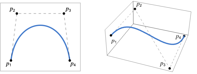
A Bézier curve and its control points in 2D:
pts = {{0, 0}, {1, 1}, {2, -1}, {3, 0}};Graphics[{BezierCurve[pts], Dashed, Gray, Line[pts], Red, Point[pts]}]A Bézier curve and its control points in 3D:
pts = {{0, 0, 0}, {1, 1, 1}, {2, -1, 1}, {3, 0, 2}}Graphics3D[{BezierCurve[pts], Dashed, Gray, Line[pts], Red, Point[pts]}]reg = BezierCurve[{{0, 0}, {1, 1}, {2, -1}}];ArcLength[reg]RegionBounds[reg]The letter "S" constructed from Bézier curves:
Graphics[{LinearGradientFilling[{StandardRed, StandardYellow}], EdgeForm[Thick], FilledCurve[BezierCurve[IconizedObject[«[image]»]]]}]Scope (26)
Basic Uses (4)
Graphics[BezierCurve[{{0, 0}, {2, 1}}]]Graphics[BezierCurve[{{-3, 0}, {6, 5}, {-6, -5}, {3, 0}}]]Graphics[BezierCurve[{{-1, 3}, {-2, 0}, {2, 0}, {1, 3}}]]Graphics[BezierCurve[{{0, 1}, {-1, 0}, {1, 0}}, SplineClosed -> True]]Graphics[{FilledCurve[BezierCurve[IconizedObject[«[image]»]]]}]Graphics[BezierCurve[IconizedObject[«[image]»]]]BezierCurve[{{-3, 0}, {6, 5}, {-6, -5}, {3, 0}}]Specifications (4)
A quadratic Bézier curve requires three control points:
Graphics[BezierCurve[{{-1, 0}, {0, 2}, {1, 0}}]]Graphics3D[BezierCurve[{{-1, 0, 0}, {0, 2, 1}, {1, 0, 0}}]]A cubic Bézier curve requires four control points:
Graphics[BezierCurve[{{-3, 0}, {6, 5}, {-6, -5}, {3, 0}}]]Graphics3D[BezierCurve[{{-3, -1, 0}, {6, 5, 5}, {-6, -5, -5}, {3, 1, 0}}]]In general, a simple degree-d Bézier curve requires (d+1) control points:
pts = {{0, 0}, {(1/3), (Sqrt[3]/2)}, {(2/3), (Sqrt[3]/2)}, {1, 0}, {(4/3), (Sqrt[3]/2)}, {(5/3), (Sqrt[3]/2)}, {2, 0}};deg = Length[pts] - 1;BezierCurve[pts, SplineDegree -> deg]Graphics[%]With fewer control points, a lower-degree curve is generated:
BezierCurve[Take[pts, 4], SplineDegree -> deg]Graphics[%]With more control points, a composite Bézier curve is generated:
BezierCurve[pts, SplineDegree -> 3]Graphics[%]Graphics[{BezierCurve[{{-2, 0}, {-1, 2}, {1, 2}, {2, 0}}]}]Graphics[{BezierCurve[{{-2, 0}, {-1, 2}, {1, 2}, {2, 0}}, SplineClosed -> True]}]Graphics (12)
Table[Graphics[{c, BezierCurve[{{0, 0}, {1, 2}, {3, 2}, {4, 0}}]}], {c, {RGBColor[0.93, 0.27, 0.27], RGBColor[0.14, 0.8, 0.14], RGBColor[0.4, 0.6, 1]}}]Bézier curves with different thicknesses:
Table[Graphics[{Thickness[i], BezierCurve[{{0, 0}, {1, 2}, {3, 2}, {4, 0}}]}], {i, {Tiny, Small, Medium, Large}}]Table[Graphics[{t, BezierCurve[{{0, 0}, {1, 2}, {3, 2}, {4, 0}}]}], {t, {Thin, Thick}}]Thickness scaled relative to the PlotRange:
Table[Graphics[{Thickness[i], BezierCurve[{{0, 0}, {1, 2}, {3, 2}, {4, 0}}]}], {i, {.005, .05, .1}}]Thickness in printer's points:
Table[Graphics[{AbsoluteThickness[i], BezierCurve[{{0, 0}, {1, 2}, {3, 2}, {4, 0}}]}], {i, {1, 5, 10}}]Table[Graphics[{Dashing[i], BezierCurve[{{0, 0}, {1, 2}, {3, 2}, {4, 0}}]}], {i, {Tiny, Small, Medium, Large}}]Table[Graphics[{d, BezierCurve[{{0, 0}, {1, 2}, {3, 2}, {4, 0}}]}], {d, {Dotted, Dashed, DotDashed}}]Opacity determines the curve transparency:
Table[Graphics[{Opacity[o], BezierCurve[{{0, 0}, {1, 2}, {3, 2}, {4, 0}}]}], {o, {0.1, 0.5, 0.9}}]EdgeForm can be used to specify the curve style when used as a boundary in a FilledCurve:
Graphics[{EdgeForm[{StandardBlue, Thick}], Opacity[0.1], FilledCurve[BezierCurve[{{0, 0}, {1, 2}, {3, 2}, {4, 0}}]]}]BezierCurve can be used as the curve for an Arrow in 2D:
Graphics[{Arrowheads[Large], Arrow[BezierCurve[{{0, 0}, {1, 2}, {3, 2}, {4, 0}}]]}]Graphics3D[{Arrowheads[Large], Arrow[BezierCurve[{{0, 0, 0}, {1, 2, 2}, {3, 2, 02}, {4, 0, 0}}]]}]In 3D, BezierCurve can be used as the curve for a Tube:
Graphics3D[{Tube[BezierCurve[{{0, 0, 0}, {1, 2, 2}, {3, 2, 02}, {4, 0, 0}}], 0.1]}]Graphics3D[{Arrowheads[0.2], Arrow[Tube[BezierCurve[{{0, 0, 0}, {1, 2, 2}, {3, 2, 02}, {4, 0, 0}}], 0.1]]}]BezierCurve can be used in GraphicsComplex:
Graphics[{GraphicsComplex[{{0, 0}, {1, 2}, {3, 2}, {4, 0}}, BezierCurve[{1, 2, 3, 4}]]}]By default, control points are assumed to be in world coordinates:
pts = {{0, 0}, {(1/4), 1}, {(3/4), 1}, {1, 0}};Table[Graphics[{BezierCurve[pts]}, Frame -> True, PlotRange -> {{0, pr}, {0, pr}}], {pr, {1, 2, 4}}]Use Scaled to specify control points relative to the PlotRange:
Table[Graphics[{BezierCurve[Map[Scaled, pts]]}, Frame -> True, PlotRange -> {{0, pr}, {0, pr}}], {pr, {4, 8, 16}}]Use ImageScaled to specify control points relative to the whole image region in 2D:
Table[Graphics[{BezierCurve[Map[ImageScaled, pts]]}, Frame -> True, PlotRange -> {{0, pr}, {0, pr}}], {pr, {4, 8, 16}}]Use Offset to apply an absolute offset to control points in 2D:
pts = {{0, 0}, {(1/4), 1}, {(3/4), 1}, {1, 0}};offsets = {{-80, 0}, {0, 0}, {80, 0}};Graphics[{Table[BezierCurve[Map[Offset[offset, #]&, pts]], {offset, offsets}]}, PlotRange -> {{-1.4, 2.4}, {-0.1, 1}}, ImageSize -> 250]Control points can be Dynamic:
DynamicModule[{z = 0, pts},
	pts = {{Dynamic[{0, z}], {1, 2}, {3, 2}, {4, 0}}};
	{Slider[Dynamic[z], {0, 4}], Graphics[{BezierCurve[pts]}]}]
Regions (6)
reg = BezierCurve[{{Subscript[c, 1], Subscript[c, 2]}, {Subscript[c, 3], Subscript[c, 4]}, {Subscript[c, 5], Subscript[c, 6]}}];RegionEmbeddingDimension[reg]RegionDimension[reg]reg = BezierCurve[{{0, 0}, {1, 2}, {3, 2}, {4, 0}}];{RegionMember[reg, {0, 0}], RegionMember[reg, {0, 1}]}reg = BezierCurve[{{0, 0}, {1, 2}, {2, 0}}];{ArcLength[reg], RegionMeasure[reg]}c = RegionCentroid[reg]Show[Region[reg], Graphics[{LightDarkSwitched[Black, White], Point[c]}]]reg = BezierCurve[{{-1, -1}, {0, 1}, {1, -1}}];{RegionDistance[reg, {-1, -1}], RegionDistance[reg, {2, 2}]}Visualize equidistance contours:
Show[Region[reg], ContourPlot[Evaluate@RegionDistance[reg, {x, y}], {x, -4, 4}, {y, -4, 3}, Contours -> {1, 2, 3}, ...], Frame -> True]reg = BezierCurve[{{-1, -1}, {0, 1}, {1, -1}}];{SignedRegionDistance[reg, {-1, -1}], SignedRegionDistance[reg, {2, 2}]}reg = BezierCurve[{{-1, -1}, {0, 1}, {1, -1}}];BoundedRegionQ[reg]bb = CoordinateBoundingBox[reg]Show[Region[reg], Graphics[{Opacity[0.1], EdgeForm[Dashed], Cuboid@@bb}]]Options (3)
SplineDegree (2)
By default, a BezierCurve with 4 or more control points will use a degree of 3:
pts = Table[{i, (-1) ^ i}, {i, 10}];{BezierCurve[Take[pts, 4]], BezierCurve[Take[pts, 10]]}With fewer control points, a lower degree is used:
{BezierCurve[Take[pts, 2]], BezierCurve[Take[pts, 3]]}Use SplineDegree to specify that a lower degree should be used:
BezierCurve[pts, SplineDegree -> 1]BezierCurve[pts, SplineDegree -> 9]For a BezierCurve with n control points, specifying a degree d where d < n-1 will give a composite Bézier curve:
pts = Table[{i, 2(-1) ^ i}, {i, 7}];Region[BezierCurve[pts, SplineDegree -> #]]& /@ {2, 3, 4}SplineClosed (1)
By default, the curve is open:
pts = {{0, -(1/2)}, {(Sqrt[3]/2), -(1/2)}, {(Sqrt[3]/2), (1/2)}, {0, (1/2)}, {-(Sqrt[3]/2), (1/2)}, {-(Sqrt[3]/2), -(1/2)}};Graphics[{BezierCurve[pts]}]Use SplineClosed to close the curve:
Graphics[{BezierCurve[pts, SplineClosed -> True]}]This is equivalent to appending the first control point to the end of the array:
Graphics[{BezierCurve[Append[pts, First[pts]]]}]Applications (6)
Fonts (4)
Fonts typically use Bézier curves to define the boundaries of glyphs:
Graphics[BezierCurve[#]]& /@ {IconizedObject[«[image]»], IconizedObject[«[image]»], IconizedObject[«[image]»]}Specify different edge styles:
glyph = FilledCurve[BezierCurve[IconizedObject[«[image]»]]];Graphics[{EdgeForm[#], FaceForm[], glyph}]& /@ {Thick, Dashed, StandardRed}Graphics[{#, glyph}]& /@ {StandardBlue, LinearGradientFilling[{StandardRed, StandardYellow}], HatchFilling[0, 1, 3]}Graphics[{#, glyph}, PlotRangePadding -> Scaled[0.05]]& /@ {DropShadowing[], Haloing[StandardYellow, 0, 5], Blurring[]}Simulate different font weights using RegionDilation:
glyph = FilledCurve[Map[List, BezierCurve /@ {IconizedObject[«[image]»], IconizedObject[«[image]»], IconizedObject[«[image]»]}]];Table[Graphics[RegionDilation[glyph, t]], {t, {0, 2}}]Table[Graphics[{Haloing[ThemeColor["Foreground"], t], glyph}, PlotRangePadding -> Scaled[.1]], {t, {0, 5}}]Simulate different font slants with ShearingTransform:
glyph = FilledCurve[Map[List, BezierCurve /@ {IconizedObject[«[image]»], IconizedObject[«[image]»], IconizedObject[«[image]»]}]];Table[Graphics[GeometricTransformation[glyph, ShearingTransform[θ , {1, 0}, {0, 1}]]], {θ, {0, 20Degree}}]Vector Graphics (2)
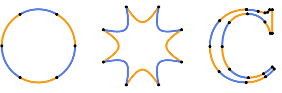
Use BezierCurve to draw shapes consisting of freeform paths:
Graphics[{BezierCurve[IconizedObject[«[image]»]]}]Use FilledCurve to style the shape interior:
Graphics[{LinearGradientFilling[{Hue[0.333, 0.8250000000000001, 0.639], Hue[0.169, 1, 0.9530000000000001]}, Top], EdgeForm[Thick], FilledCurve[BezierCurve[IconizedObject[«[image]»]]]}]Use multiple Bézier curves to draw more complex shapes:
curves = BezierCurve /@ {IconizedObject[«[image]»], IconizedObject[«[image]»], IconizedObject[«[image]»], IconizedObject[«[image]»], IconizedObject[«[image]»]};Graphics[curves]Graphics[{FilledCurve[List /@ curves], RGBColor[0.9058724017188509, 0.13725482819401516, 0., 1.], FilledCurve[curves[[1]]]}]Properties & Relations (14)
A BezierCurve with degree 1 is equivalent to Line:
pts = {{0, -1}, {2, 1}, {4, -1}, {6, 1}};Graphics /@ {BezierCurve[pts, SplineDegree -> 1], Line[pts]}A BezierCurve is a special case of BSplineCurve:
pts = {{-3, 0}, {6, 5}, {-6, -5}, {3, 0}};Graphics /@ {BezierCurve[pts], BSplineCurve[pts]}Use RegionConvert to get the equivalent BSplineCurve:
RegionConvert[BezierCurve[pts], "Spline"]BezierSurface is a higher-dimensional form of BezierCurve that takes a rectangular array of control points:
pts = (| | | | |
| ---------- | ----------- | ----------- | ----------- |
| {0, 0, 7} | {0, 3, 10} | {0, 7, 10} | {0, 10, 7} |
| {3, 0, 10} | {3, 3, 14} | {3, 7, 14} | {3, 10, 10} |
| {7, 0, 10} | {7, 3, 14} | {7, 7, 14} | {7, 10, 10} |
| {10, 0, 7} | {10, 3, 10} | {10, 7, 10} | {10, 10, 7} |);Graphics3D[BezierSurface[pts]]The boundary edges of a BezierSurface are formed from four Bézier curves:
bc = Map[BezierCurve, {pts[[1]], pts[[-1]], pts[[All, 1]], pts[[All, -1]]}];Graphics3D[{BezierSurface[pts], Thick, StandardRed, bc}]All isoparametric curves on a BezierSurface are valid Bézier curves:
uc = Table[BezierCurve[Map[#[u]&, Map[BezierFunction, pts]]], {u, 0, 1, 1 / 5}];
vc = Table[BezierCurve[Map[#[v]&, Map[BezierFunction, Transpose[pts]]]], {v, 0, 1, 1 / 5}];Graphics3D[{BezierSurface[pts], Thick, RGBColor[0.14, 0.8, 0.14], uc, RGBColor[0.4, 0.6, 1], vc}]A Circle can be closely approximated with a composite BezierCurve:
Region /@ {BezierCurve[IconizedObject[«[image]»]], Circle[]}The approximation error is minor:
RegionHausdorffDistance@@%BezierCurve always interpolates its first and last control point:
pts = {{0, -1}, {1, 2}, {2, -2}, {3, 1}};Graphics[{BezierCurve[pts], Red, Point[{First[pts], Last[pts]}]}]A Bézier curve lies in the convex hull of its control points:
pts = {{0, -1}, {2, 1}, {4, -1}, {6, 1}, {4, 2}};hull = ConvexHullMesh[pts, MeshCellStyle -> {0 -> Red, 2 -> Opacity[1 / 4]}];Show[hull, Region[BezierCurve[pts, SplineDegree -> 4]]]In 3D, a Bézier curve with coplanar control points lies in the same plane as its points:
pts = {{-3, -1, 0}, {6, 10, 0}, {-6, -10, 0}, {3, 1, 0}};pts//CoplanarPointsGraphics3D[{InfinitePlane[Take[pts, 3]], BezierCurve[pts]}, Lighting -> "Accent", ViewPoint -> #]& /@ {2{1, -1, 1}, Front, Top}BezierFunction gives the position on a BezierCurve corresponding to a specific parameter value:
pts = {{-3, 0}, {6, 5}, {-6, -5}, {3, 0}};bfunc = BezierFunction[pts]positions = Table[bfunc[u], {u, 0, 1, 1 / 10}];Graphics[{BezierCurve[pts], StandardRed, PointSize[0.02], Point[positions]}]A Bézier curve can be constructed using Bernstein polynomials to take a weighted sum of its control points:
pts = {{0, -1}, {1, 1}, {2, -1}, {3, 1}};bezier[t_] := Sum[BernsteinBasis[3, i, t] * pts[[i + 1]], {i, 0, 3}]GraphicsRow[{ParametricPlot[bezier[t], {t, 0, 1}, Frame -> True, Axes -> False], Graphics[BezierCurve[pts], Frame -> True]}, ImageSize -> 400]Use BernsteinBasis to visualize the weight of each control point along the curve:
weights = Table[BernsteinBasis[3, i, t], {i, 0, 3}];Plot[weights, {t, 0, 1}, PlotLegends -> {"SubscriptBox[p, 1]", "SubscriptBox[p, 2]", "SubscriptBox[p, 3]", "SubscriptBox[p, 4]"}]A Bézier curve is affine invariant:
pts = {{0, -1}, {2, 2}, {4, -2}, {6, 1}};A = AffineTransform[{{{1, 1}, {0, 2}}, {1, 2}}];{Graphics[GeometricTransformation[BezierCurve[pts], A], Frame -> True],
Graphics[BezierCurve[A[pts]], Frame -> True]}Averaging the control points of two Bézier curves is equivalent to averaging the curves themselves:
pts1 = {{0, -1}, {2, 1}, {4, 2}, {6, 2}};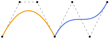
pts2 = {{2, -1}, {3, 1}, {4, -1}, {6, 0}};Graphics[{Thick, RGBColor[0.4, 0.6, 1], BezierCurve[pts1], RGBColor[0.98, 0.56, 0.17], BezierCurve[pts2], RGBColor[0.93, 0.27, 0.27], BezierCurve[Mean[{pts1, pts2}]]}, Frame -> True]ParametricPlot[{BezierFunction[pts1][t], BezierFunction[pts2][t], Mean[{BezierFunction[pts1][t], BezierFunction[pts2][t]}]}, {t, 0, 1}, Frame -> True, Axes -> False, PlotStyle -> {RGBColor[0.4, 0.6, 1], RGBColor[0.98, 0.56, 0.17], RGBColor[0.93, 0.27, 0.27]}]A composite Bézier curve may not be smooth at the point where two segments meet:
pts = {{0, 0}, {1, -1}, {3, -1}, {3, 0}, {4, 1}, {5, 1}, {6, 0}};Graphics[{BezierCurve[pts], Dashed, Gray, Line[pts], Red, Point[pts]}]Set points adjacent to the boundary to be collinear to guarantee composite Bézier curve:
pts[[5, 1]] = 3;Graphics[{BezierCurve[pts], Dashed, Gray, Line[pts], Red, Point[pts]}]A Bézier curve can be elevated to an equivalent curve of any higher degree:
pts = {{0, 0}, {2, 3}, {4, 0}};elevate[pts_] := With[...]epts = Table[Nest[elevate, pts, d], {d, 0, 3}];Graphics /@ Table[{BezierCurve[epts[[i]], SplineDegree -> i + 2], Dashed, Gray, Line[epts[[i]]], Red, Point[epts[[i]]]}, {i, Length[epts]}]SubdivisionRegion generates smooth surfaces from control meshes instead of control points:
Region /@ {SubdivisionRegion[[image]], BezierCurve[IconizedObject[«[image]»]]}Interactive Examples (2)
Column[{Manipulate[DynamicModule[{},
	$curve = BezierCurve[pts, SplineDegree -> d, SplineClosed -> c];
	Graphics[{$curve, Dashed, Opacity[0.5], Line[pts]}, PlotRange -> 5, Frame -> True, ImageSize -> 250]], {{pts, {{-4, -4}, {-3, 4}, {3, -4}, {4, 4}}}, Locator, LocatorAutoCreate -> True}, {{d, 3, "degree"}, 2, 6, 1}, {{c, False, "closed"}, {False, True}}], Button["Copy Curve to Clipboard", CopyToClipboard[$curve]]}]
Smoothly interpolate between two simple Bézier curves:
interpolateCurves[pts1_, pts2_] :=
Manipulate[Graphics[{BezierCurve[pts1(1 - t) + pts2 t], Opacity[0.25], Dashed, BezierCurve[pts1], BezierCurve[pts2]}], {t, 0, 1}]interpolateCurves[{...}, {...}]interpolateCurves@@{{...}, {...}}Text
Wolfram Research (2008), BezierCurve, Wolfram Language function, https://reference.wolfram.com/language/ref/BezierCurve.html.
CMS
Wolfram Language. 2008. "BezierCurve." Wolfram Language & System Documentation Center. Wolfram Research. https://reference.wolfram.com/language/ref/BezierCurve.html.
APA
Wolfram Language. (2008). BezierCurve. Wolfram Language & System Documentation Center. Retrieved from https://reference.wolfram.com/language/ref/BezierCurve.html