


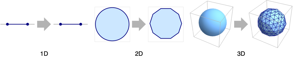
BoundaryDiscretizeRegion
discretizes the region reg into a BoundaryMeshRegion.
BoundaryDiscretizeRegion[reg,{{xmin,xmax},…}]
restricts to the bounds ![]() .
.
Details and Options
- BoundaryDiscretizeRegion is also known as boundary evaluation.
- BoundaryDiscretizeRegion effectively discretizes the boundaries of the full-dimensional parts of a region reg.
- The region reg can be anything that is ConstantRegionQ and RegionEmbeddingDimension less or equal to 3.
- BoundaryDiscretizeRegion has the same options as BoundaryMeshRegion, with the following additions and changes:
-
AccuracyGoal Automatic digits of accuracy sought MaxCellMeasure Automatic maximum cell measure Method Automatic method to use PerformanceGoal $PerformanceGoal whether to consider speed or quality PrecisionGoal Automatic digits of precision sought - With AccuracyGoal->a and PrecisionGoal->p, an attempt will be made to keep the maximum distance between the region reg or the discretized region dreg and any point in RegionSymmetricDifference[reg,dreg] to less than
 , where
  is the length of the diagonal of the bounding box.
 - With MaxCellMeasure->m where m>0, the cell measure in the boundary dimension d-1 where d is the region dimension will be limited to m. Measure limits for specific dimensions may be specified with MaxCellMeasure->{…,di->mi,…}.
Examples
open all close allBasic Examples (2)
Get a discretized boundary representation for a disk:
BoundaryDiscretizeRegion[Disk[]]Restrict to the first quadrant:
BoundaryDiscretizeRegion[Disk[], {{0, 1}, {0, 1}}]Get a discretized boundary representation for a ball:
BoundaryDiscretizeRegion[Ball[]]Restrict to the first orthant:
BoundaryDiscretizeRegion[Ball[], {{0, 1}, {0, 1}, {0, 1}}]Scope (24)
Regions in 1D (5)
Line and Interval are full-dimensional regions in 1D:
BoundaryDiscretizeRegion[Interval[{1, 3}]]BoundaryDiscretizeRegion[Line[Transpose@{List /@ Range[1, 20, 2], List /@ Range[2, 20, 2]}]]An ImplicitRegion is 1D if it has one variable:
BoundaryDiscretizeRegion[ImplicitRegion[Abs[Sin[x]] ≤ 3 / 4, {{x, 0, 10}}]]The discretization can be clipped to a specified range:
ℛ = ImplicitRegion[Abs[Sin[x]] ≤ 3 / 4, {x}];BoundaryDiscretizeRegion[ℛ, {{0, 10}}]A ParametricRegion is 1D if it has only one function:
BoundaryDiscretizeRegion[ParametricRegion[{t + 5}, {{t, 0, 10}}]]The discretization can be clipped to a specified range:
ℛ = ParametricRegion[{t + 5}, {{t, 0, ∞}}];
BoundedRegionQ[ℛ]
Because this region is unbounded, clip it to discretize:
BoundaryDiscretizeRegion[ℛ, {{0, 10}}]A BooleanRegion in 1D:
BoundaryDiscretizeRegion[BooleanRegion[Xor, {Line[{{-2}, {1}}], Line[{{-1}, {2}}]}]]Boundary discretization can only represent full-dimensional region components:
ℛ = ImplicitRegion[x == 0 || x ≥ 1, {{x, 0, 3}}];BoundaryDiscretizeRegion[ℛ]Use DiscretizeRegion to discretize lower-dimensional components as well:
DiscretizeRegion[ℛ]Regions in 2D (8)
Rectangle, Disk, and Simplex are special regions that can be full dimensional in 2D:
BoundaryDiscretizeRegion[Rectangle[]]Disk:
BoundaryDiscretizeRegion[Disk[]]BoundaryDiscretizeRegion[Simplex[2]]An ImplicitRegion is 2D if it has two variables:
BoundaryDiscretizeRegion[ImplicitRegion[x ^ 2 - y ^ 2 ≤ 1, {{x, -3, 3}, {y, -3, 3}}]]For an unbounded region, clip the discretization to a specified range:
ℛ = ImplicitRegion[x ^ 2 - y ^ 2 ≤ 1, {x, y}];
BoundedRegionQ[ℛ]BoundaryDiscretizeRegion[ℛ, {{-3, 3}, {-3, 3}}]A ParametricRegion is in 2D if it has two functions:
BoundaryDiscretizeRegion[ParametricRegion[{{t, s (1 - t ^ 2)}, -1 ≤ s ≤ 1 && -1 ≤ t ≤ 1}, {s, t}]]BoundaryDiscretizeRegion[ParametricRegion[{{t, s (1 - t ^ 2)}, -1 ≤ s ≤ 1 && -1 ≤ t ≤ 1}, {s, t}], {{-1, 1}, {-2 / 3, 2 / 3}}]A region in 2D with parameters constrained to a unit disk:
BoundaryDiscretizeRegion[ParametricRegion[{{s, s t}, s ^ 2 + t ^ 2 ≤ 1}, {s, t}]]Parameters constrained to a rectangle:
BoundaryDiscretizeRegion[ParametricRegion[{{s, s t}, Element[{s, t}, Rectangle[{-1, -1}, {1, 1}]]}, {s, t}]]Given two exact regions, ParametricRegion can be used to represent their Minkowski sum:
r1 = Disk[{0, 0}, 1 / 2];
r2 = Polygon[{{0, 0}, {3, -1}, {1, 0}, {3, 1}}];
pr = ParametricRegion[{{x1 + x2, y1 + y2}, {x1, y1}∈r1 && {x2, y2}∈r2}, {x1, x2, y1, y2}];
BoundaryDiscretizeRegion[pr]
A RegionUnion in 2D:
BoundaryDiscretizeRegion[RegionUnion[Disk[{0, 0}, 1], Disk[{1, 0}, 1]]]A region can include components of different dimensions:
ℛ = ImplicitRegion[x ^ 2 + y ^ 2 ≤ 1 || x == y, {{x, -2, 2}, {y, -2, 2}}];
DiscretizeRegion[ℛ]
The boundary discretization can only represent full-dimensional components, however:
BoundaryDiscretizeRegion[ℛ]
A polygon with GeoGridPosition:
ℛ = Polygon[GeoGridPosition[{{{-0.9950503945490105, 1.2366760550756015},
   {-0.9952074890903578, 1.2369207053693891}, {-0.9952196732768064, 1.2369073327446167},
   {-0.9953160063787643, 1.236848436956935}, {-0.9954141759436825, 1.2369993898475449},
   {-0. ... 197645333103}, {-0.9949098578570917, 1.2368130881428654},
   {-0.9948663952535768, 1.2367477711687371}, {-0.9948714472169538, 1.2367426500757825},
{-0.9949211061652593, 1.2367089232486177}, {-0.9949439717990124, 1.236746107097628}}}, "Bonne"]];BoundaryDiscretizeRegion[ℛ]Regions in 3D (5)
Cuboid, Ellipsoid, and Simplex are special regions that can be full dimensional in 3D:
BoundaryDiscretizeRegion[Cuboid[{0, 0, 0}, {1, 1, 1}]]BoundaryDiscretizeRegion[Ellipsoid[{0, 0, 0}, {{5, 2, 3}, {2, 3, 2}, {3, 2, 5}}]]BoundaryDiscretizeRegion[Simplex[3]]An ImplicitRegion is 3D if it has precisely three variables:
BoundaryDiscretizeRegion[ImplicitRegion[(x ^ 2 + (9 / 4)y ^ 2 + z ^ 2 - 1) ^ 3 - x ^ 2z ^ 3 - (9 / 80)y ^ 2z ^ 3 ≤ 0, {x, y, z}]]ℛ = ImplicitRegion[x ^ 2 + y ^ 2 + z ^ 2 ≤ 1, {x, y, z}];
BoundaryDiscretizeRegion[ℛ, {{-3 / 4, 3 / 4}, {-3 / 4, 3 / 4}, {-3 / 4, 3 / 4}}]A ParametricRegion is in 3D if it has precisely three functions:
BoundaryDiscretizeRegion[ParametricRegion[{x, y, z + x * y}, {{x, -1, 1}, {y, -1, 1}, {z, -1, 1}}]]A solid in 3D generated with the parameters constrained to the unit ball:
BoundaryDiscretizeRegion[ParametricRegion[{{x, y, z + y * x}, x ^ 2 + y ^ 2 + z ^ 2 <= 1}, {x, y, z}]]A region can include components of different dimensions:
ℛ = ImplicitRegion[x ^ 2 + y ^ 2 + z ^ 2 ≤ 1 || x + y + z == 0, {{x, -2, 2}, {y, -2, 2}, {z, -2, 2}}];
DiscretizeRegion[ℛ]
The boundary discretization can only represent full-dimensional components, however:
BoundaryDiscretizeRegion[ℛ]
Detail (2)
The measure of cells in the discretization can be controlled using MaxCellMeasure:
Ω = ImplicitRegion[Abs[x] + Abs[y] ≥ 1, {{x, -2, 2}, {y, -2, 2}}];HighlightMesh[BoundaryDiscretizeRegion[Ω, MaxCellMeasure -> #], 0]& /@ {Automatic, 5, 1, 1 / 5}By default, when given as a number, it applies to the boundary dimension:
HighlightMesh[BoundaryDiscretizeRegion[Ω, MaxCellMeasure -> .5], 0]With area a, a length l is computed so that triangles with sides of length l will have area a:
HighlightMesh[bmr = BoundaryDiscretizeRegion[Ω, MaxCellMeasure -> {"Area" -> .1}], 0]Using TriangulateMesh with the same specification will maintain quality near the edge:
TriangulateMesh[bmr, MaxCellMeasure -> {"Area" -> .1}]For nonlinear regions, the measure of boundary cells depends on several options:
Ω = Disk[{1, 2}, {3, 4}, {5, 6}];
HighlightMesh[BoundaryDiscretizeRegion[Ω], 0]
The length of any segment may be controlled by MaxCellMeasure:
HighlightMesh[BoundaryDiscretizeRegion[Ω, MaxCellMeasure -> {"Length" -> #}], 0]& /@ {5, 1, 1 / 5}The default PrecisionGoal is chosen to be a value so that curves appear as visually smooth:
HighlightMesh[BoundaryDiscretizeRegion[Ω, PrecisionGoal -> #], 0]& /@ {Automatic, 1, 4}MaxCellMeasure->∞ may be used to base the boundary measure on precision:
HighlightMesh[BoundaryDiscretizeRegion[Ω, MaxCellMeasure -> ∞, PrecisionGoal -> #], 0]& /@ {Automatic, 1, 2, 3, 4}PrecisionGoal->None may be used to base the boundary measure on MaxCellMeasure:
HighlightMesh[BoundaryDiscretizeRegion[Ω, MaxCellMeasure -> {"Length" -> #}, PrecisionGoal -> None], 0]& /@ {5, 1, 1 / 5}AccuracyGoal->a may be used to specify an absolute tolerance ![]() :
:
HighlightMesh[BoundaryDiscretizeRegion[Ω, MaxCellMeasure -> ∞, PrecisionGoal -> None, AccuracyGoal -> #], 0]& /@ {0, 1, 2, 3}The default is for MaxCellMeasure to apply to the boundary dimension:
HighlightMesh[BoundaryDiscretizeRegion[Ω, MaxCellMeasure -> #], 0]& /@ {10, 1, 1 / 10}The measure on the boundary may be further restricted by approximation requirements:
HighlightMesh[BoundaryDiscretizeRegion[Ω, MaxCellMeasure -> #, AccuracyGoal -> 4], 0]& /@ {10, 1, 1 / 10}Quality (4)
The measure of cells in the discretization can be controlled using MaxCellMeasure:
BoundaryDiscretizeRegion[Disk[], MaxCellMeasure -> #]& /@ {1, 0.1, 0.01}By default, this controls the measure of the edges:
Max[AnnotationValue[{#, 1}, MeshCellMeasure]]& /@ %Use AccuracyGoal to ensure the discretized boundary is close to the exact boundary:
{ℛ1, ℛ2} = BoundaryDiscretizeRegion[Disk[], AccuracyGoal -> #]& /@ {2, 5}The discretization with the higher AccuracyGoal is closer to the true boundary:
1 - Max[Norm[#]& /@ AnnotationValue[{#, {1}}, MeshCellCentroid]]& /@ {ℛ1, ℛ2}Use PrecisionGoal to ensure the discretized boundary is close to the exact boundary:
{ℛ1, ℛ2} = BoundaryDiscretizeRegion[Disk[], PrecisionGoal -> #]& /@ {2, 5}The discretization with the higher PrecisionGoal is closer to the true boundary:
1 - Max[Norm[#]& /@ AnnotationValue[{#, {1}}, MeshCellCentroid]]& /@ {ℛ1, ℛ2}Set PerformanceGoal to "Quality" for a high-quality discretization:
ℛ = ImplicitRegion[-1 + 2 x^2 ≤ y ≤ x^2, {{x, -1, 1}, {y, -1, 1}}];BoundaryDiscretizeRegion[ℛ, PerformanceGoal -> "Quality"]Or to "Speed" for a faster discretization that may be of lower quality:
BoundaryDiscretizeRegion[ℛ, PerformanceGoal -> "Speed"]Options (24)
AccuracyGoal (1)
Ensure that the discretized boundary representation is close to the boundary:
bmr = BoundaryDiscretizeRegion[Disk[], AccuracyGoal -> 2]The largest deviation from the true disk is at the centers of the segments:
ListPlot[err = Map[{ArcTan@@#, Norm[#] - 1}&, AnnotationValue[{bmr, 1}, MeshCellCentroid]]]With a larger accuracy goal, the error is reduced by using more points:
bmr = BoundaryDiscretizeRegion[Disk[], AccuracyGoal -> 3];
ListPlot[err = Map[{ArcTan@@#, Norm[#] - 1}&, AnnotationValue[{bmr, 1}, MeshCellCentroid]]]
MaxCellMeasure (2)
With MaxCellMeasure->m, boundary cell size is less than or equal to ![]() :
:
bmr = BoundaryDiscretizeRegion[Disk[{0, 0}, {2, 1}], MaxCellMeasure -> .1]This gives the lengths of the segments:
Histogram[AnnotationValue[{bmr, 1}, MeshCellMeasure]]In 3D, the area of faces is controlled by MaxCellMeasure:
bmr = BoundaryDiscretizeRegion[Ellipsoid[{0, 0, 0}, {3, 2, 1}], MaxCellMeasure -> .1]This gives the areas of the faces:
Histogram[AnnotationValue[{bmr, 2}, MeshCellMeasure]]The lengths of edges can be controlled by setting a max measure for "Length":
bmr = BoundaryDiscretizeRegion[Ellipsoid[{0, 0, 0}, {3, 2, 1}], MaxCellMeasure -> {"Length" -> 0.3}]This gives the lengths of the edges:
Histogram[AnnotationValue[{bmr, 1}, MeshCellMeasure]]MeshCellHighlight (3)
MeshCellHighlight allows you to specify highlighting for parts of a BoundaryMeshRegion:
BoundaryDiscretizeRegion[Disk[], MeshCellHighlight -> {{1, All} -> Red, {0, All} -> Black}]By making faces transparent, the internal structure of a 3D BoundaryMeshRegion can be seen:
BoundaryDiscretizeRegion[Cuboid[{0, 0, 0}, {1, 1, 1}], MeshCellHighlight -> {{2, All} -> Opacity[0.5, Orange]}]Individual cells can be highlighted using their cell index:
BoundaryDiscretizeRegion[Simplex[2], MaxCellMeasure -> 1, MeshCellHighlight -> {{1, 1} -> {Thick, Red}, {1, 2} -> {Dashed, Black}}]BoundaryDiscretizeRegion[Simplex[2], MaxCellMeasure -> 1, MeshCellHighlight -> {Line[{1, 2}] -> {Thick, Red}, Line[{2, 4}] -> {Dashed, Black}}]MeshCellLabel (3)
MeshCellLabel can be used to label parts of a BoundaryMeshRegion:
BoundaryDiscretizeRegion[Interval[{1, 3}], MeshCellLabel -> {0 -> "Index"}]Label the vertices and edges of a rectangle:
BoundaryDiscretizeRegion[Rectangle[], MaxCellMeasure -> 1, MeshCellLabel -> {0 -> "Index", 1 -> "Index"}]Individual cells can be labeled using their cell index:
BoundaryDiscretizeRegion[Interval[{1, 3}], MeshCellLabel -> {{0, 1} -> "x", {0, 2} -> "y"}]BoundaryDiscretizeRegion[Interval[{1, 3}], MeshCellLabel -> {Point[1] -> "x", Point[2] -> "y"}]MeshCellMarker (1)
MeshCellMarker can be used to assign values to parts of a BoundaryMeshRegion:
BoundaryDiscretizeRegion[Rectangle[], MeshCellMarker -> {{0, 1} -> 1, {0, 2} -> 2}]Use MeshCellLabel to show the markers:
BoundaryDiscretizeRegion[Rectangle[], MeshCellMarker -> {{0, 1} -> 1, {0, 2} -> 2}, MeshCellLabel -> {0 -> "Marker"}]MeshCellShapeFunction (2)
MeshCellShapeFunction allows you to specify functions for parts of a BoundaryMeshRegion:
BoundaryDiscretizeRegion[Rectangle[], MaxCellMeasure -> 1, MeshCellShapeFunction -> {0 -> (Disk[#, .1]&)}]Individual cells can be drawn using their cell index:
BoundaryDiscretizeRegion[Rectangle[], MaxCellMeasure -> 1, MeshCellShapeFunction -> {{0, 1} -> (Disk[#, .1]&), {0, 2} -> (Disk[#, {.1, .2}]&)}]BoundaryDiscretizeRegion[Rectangle[], MaxCellMeasure -> 1, MeshCellShapeFunction -> {Point[1] -> (Disk[#, .1]&), Point[2] -> (Disk[#, {.1, .2}]&)}]MeshCellStyle (3)
MeshCellStyle allows you to specify styling for parts of a BoundaryMeshRegion:
BoundaryDiscretizeRegion[Disk[], MeshCellStyle -> {{1, All} -> Red, {0, All} -> Black}]By making faces transparent, the internal structure of a 3D BoundaryMeshRegion can be seen:
BoundaryDiscretizeRegion[Cuboid[{0, 0, 0}, {1, 1, 1}], MeshCellStyle -> {{2, All} -> Opacity[0.5, Orange]}]Individual cells can be highlighted using their cell index:
BoundaryDiscretizeRegion[Simplex[2], MaxCellMeasure -> 1, MeshCellStyle -> {{1, 1} -> Directive[Thick, Red], {1, 2} -> Directive[Dashed, Black]}]BoundaryDiscretizeRegion[Simplex[2], MaxCellMeasure -> 1, MeshCellStyle -> {Line[{1, 2}] -> Directive[Thick, Red], Line[{2, 4}] -> Directive[Dashed, Black]}]Method (6)
The "Continuation" method uses a curve continuation method that can in many cases resolve corners, cusps, and sharp changes quite well:
ℛ = ImplicitRegion[-1 + 2 x^2 ≤ y ≤ x^2, {{x, -1, 1}, {y, -1, 1}}];BoundaryDiscretizeRegion[ℛ, Method -> "Continuation"]The "RegionPlot" method is based on improving output from RegionPlot and can sometimes be faster:
ℛ = ImplicitRegion[-1 + 2 x^2 ≤ y ≤ x^2, {{x, -1, 1}, {y, -1, 1}}];BoundaryDiscretizeRegion[ℛ, Method -> "RegionPlot"]The "Boolean" method is optimized for Boolean regions:
BoundaryDiscretizeRegion[RegionUnion[Disk[{0, 0}, 1], Disk[{1, 0}, 1]], Method -> "Boolean"]The "DiscretizeGraphics" method is optimized for graphics primitives:
BoundaryDiscretizeRegion[Disk[], Method -> "DiscretizeGraphics"]The "RegionPlot3D" method for 3D regions is based on RegionPlot3D:
BoundaryDiscretizeRegion[Ball[], Method -> "RegionPlot3D"]The "ContourPlot3D" method for 3D regions is based on ContourPlot3D:
BoundaryDiscretizeRegion[Ball[], Method -> "ContourPlot3D"]PlotTheme (2)
PrecisionGoal (1)
Ensure that the discretized boundary representation is close to the boundary:
bmr = BoundaryDiscretizeRegion[Disk[], PrecisionGoal -> 2]The largest deviation from the true disk is at the centers of the segments:
ListPlot[err = Map[{ArcTan@@#, Norm[#] - 1}&, AnnotationValue[{bmr, 1}, MeshCellCentroid]]]With a larger accuracy goal, the error is reduced by using more points:
bmr = BoundaryDiscretizeRegion[Disk[], AccuracyGoal -> 3];
ListPlot[err = Map[{ArcTan@@#, Norm[#] - 1}&, AnnotationValue[{bmr, 1}, MeshCellCentroid]]]
Applications (2)
Visualize LaminaData:
f = LaminaData["Salinon", "Region"]Discretize and visualize the region:
BoundaryDiscretizeRegion[f[1, .5]]Visualize SolidData:
f = SolidData["CylindricalHalfShell", "Region"]Discretize and visualize the region:
BoundaryDiscretizeRegion[f[1, .5, 2]]Properties & Relations (5)
The output of BoundaryDiscretizeRegion is a BoundaryMeshRegion:
ℛ = BoundaryDiscretizeRegion[Disk[]]BoundaryMeshRegionQ[ℛ]Given a boundary discretization, TriangulateMesh can discretize the interior:
{ℛ = BoundaryDiscretizeRegion[Disk[]], TriangulateMesh[ℛ]}The boundary discretization represents the regular closure of a region:
ℛ = RegionUnion[Disk[], Line[{{-1, -1}, {1, 1}}]];BoundaryDiscretizeRegion[ℛ]The lower-dimensional component is lost, but can be represented by DiscretizeRegion:
DiscretizeRegion[ℛ]BoundaryDiscretizeRegion can discretize a region with holes:
BoundaryDiscretizeRegion[ImplicitRegion[1 ≤ x^2 + y^2 ≤ 4, {x, y}]]BoundaryDiscretizeRegion can discretize a region with disjoint components:
BoundaryDiscretizeRegion[ImplicitRegion[Sin[x y] ≤ 0.2, {x, y}], {{0, 5}, {0, 5}}]Text
Wolfram Research (2014), BoundaryDiscretizeRegion, Wolfram Language function, https://reference.wolfram.com/language/ref/BoundaryDiscretizeRegion.html (updated 2015).
CMS
Wolfram Language. 2014. "BoundaryDiscretizeRegion." Wolfram Language & System Documentation Center. Wolfram Research. Last Modified 2015. https://reference.wolfram.com/language/ref/BoundaryDiscretizeRegion.html.
APA
Wolfram Language. (2014). BoundaryDiscretizeRegion. Wolfram Language & System Documentation Center. Retrieved from https://reference.wolfram.com/language/ref/BoundaryDiscretizeRegion.html