


DiscretizeRegion
DiscretizeRegion[reg]
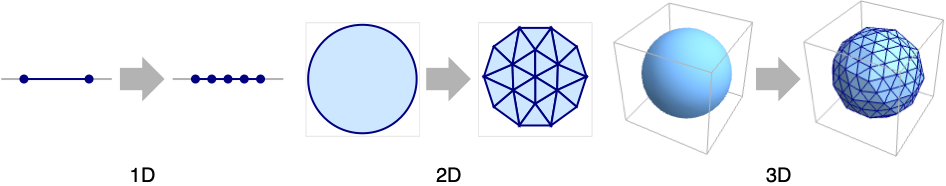
discretizes a region reg into a MeshRegion.
DiscretizeRegion[reg,{{xmin,xmax},…}]
restricts to the bounds ![]() .
.
Details and Options
- DiscretizeRegion is also known as mesh generation and grid generation.
- DiscretizeRegion discretizes the interior and boundaries of the region reg.
- In particular, DiscretizeRegion will attempt to discretize lower-dimensional parts of reg.
- The region reg can be anything that is ConstantRegionQ and RegionEmbeddingDimension less than or equal to 3.
- DiscretizeRegion has the same options as MeshRegion, with the following additions and changes:
-
AccuracyGoal Automatic digits of accuracy sought MaxCellMeasure Automatic maximum cell measure MeshQualityGoal Automatic quality goal for mesh cells Method Automatic method to use MeshRefinementFunction None function that returns True if a mesh cell needs refinement PerformanceGoal $PerformanceGoal whether to consider speed or quality PrecisionGoal Automatic digits of precision sought - With MeshRefinementFunction->f, the function f[vlist,m] is applied to each simplex created, where vlist is a list of the vertices and m is the measure. If f[vlist,m] returns True, the simplex will be refined.
- With AccuracyGoal->a and PrecisionGoal->p, an attempt will be made to keep the maximum distance between the region reg or the discretized region dreg and any point in RegionSymmetricDifference[reg,dreg] to less than
 , where
  is the length of the diagonal of the bounding box.
Examples
open all close allBasic Examples (3)
Discretize 1D embedded regions:
DiscretizeRegion[Interval[{-2, -1}, {1, 2}]]DiscretizeRegion[ImplicitRegion[Sin[x] ≤ 1 / 2, {x}], {{0, 50}}]DiscretizeRegion[ImplicitRegion[Sin[x] ≤ 1 / 2 || Sin[x] == 9 / 10, {x}], {{0, 10}}]Discretize 2D embedded regions:
DiscretizeRegion[Disk[]]Restrict to the first quadrant:
DiscretizeRegion[Disk[], {{0, 1}, {0, 1}}]DiscretizeRegion[ImplicitRegion[x ^ 2 - y ^ 2 ≤ 1 || x ^ 2 + y ^ 2 == 4, {x, y}], {{-2, 2}, {-2, 2}}]Discretize 3D embedded regions:
DiscretizeRegion[Cylinder[]]Restrict to the first orthant:
DiscretizeRegion[Ball[], {{0, 1}, {0, 1}, {0, 1}}]DiscretizeRegion[ImplicitRegion[x ^ 2 + y ^ 2 - z ^ 2 ≤ 1, {x, y, z}], {{-2, 2}, {-2, 2}, {-2, 2}}]Scope (30)
Regions in 1D (5)
Point and Line are special regions that can exist in 1D:
DiscretizeRegion[Point[List /@ Range[10]]]Line:
DiscretizeRegion[Line[Transpose@{List /@ Range[1, 20, 2], List /@ Range[2, 20, 2]}]]An ImplicitRegion is 1D if it has only one variable:
DiscretizeRegion[ImplicitRegion[Abs[Sin[x]] ≤ 3 / 4, {{x, 0, 10}}]]Because this region is unbounded, clip it to discretize:
ℛ = ImplicitRegion[Abs[Sin[x]] ≤ 3 / 4, {x}];DiscretizeRegion[ℛ, {{0, 10}}]A ParametricRegion is 1D if it has only one function:
DiscretizeRegion[ParametricRegion[{t + 5}, {{t, 0, 10}}]]The discretization can be clipped to a specified range:
ℛ = ParametricRegion[{t + 5}, {{t, 0, ∞}}];
BoundedRegionQ[ℛ]
Because this region is unbounded, clip it to discretize:
DiscretizeRegion[ℛ, {{0, 10}}]A BooleanRegion in 1D:
DiscretizeRegion[BooleanRegion[Xor, {Line[{{-2}, {1}}], Line[{{-1}, {2}}]}]]A region can include components of different dimensions:
DiscretizeRegion[ImplicitRegion[x == 0 || x ≥ 1, {{x, 0, 3}}]]Separate the components by dimension:
DimensionalMeshComponents[%]Regions in 2D (8)
Point, Circle, and Rectangle are special regions that can exist in 2D:
DiscretizeRegion[Point[Tuples[{0, 1, 2, 3}, 2]]]Circle is 1D, but embedded in 2D:
DiscretizeRegion[Circle[]]Rectangle is 2D:
DiscretizeRegion[Rectangle[]]An ImplicitRegion is 2D if it has two variables. A 1D region is typically an equation:
DiscretizeRegion[ImplicitRegion[x ^ 2 - y ^ 2 == 1, {{x, -3, 3}, {y, -3, 3}}]]A 2D region is typically a combination of inequalities:
DiscretizeRegion[ImplicitRegion[x ^ 2 - y ^ 2 ≤ 1, {{x, -3, 3}, {y, -3, 3}}]]For an unbounded region, clip the discretization to a specified range:
ℛ = ImplicitRegion[x ^ 2 - y ^ 2 ≤ 1, {x, y}];
BoundedRegionQ[ℛ]DiscretizeRegion[ℛ, {{-3, 3}, {-3, 3}}]A ParametricRegion is 2D if it has two functions. A 1D region has one parameter:
DiscretizeRegion[ParametricRegion[{Cos[4 t], Sin[3 t]}, t]]A 2D region has two parameters:
DiscretizeRegion[ParametricRegion[{{t, s (1 - t ^ 2)}, -1 ≤ s ≤ 1 && -1 ≤ t ≤ 1}, {s, t}]]DiscretizeRegion[ParametricRegion[{{t, s (1 - t ^ 2)}, -1 ≤ s ≤ 1 && -1 ≤ t ≤ 1}, {s, t}], {{-1, 1}, {-2 / 3, 2 / 3}}]A 2D parametric region with parameters constrained to a unit disk:
DiscretizeRegion[ParametricRegion[{{s, s t}, s ^ 2 + t ^ 2 ≤ 1}, {s, t}]]When the parameters are constrained to just the unit circle, the result is 1D:
DiscretizeRegion[ParametricRegion[{{s, s t}, s ^ 2 + t ^ 2 == 1}, {s, t}]]Parameters may be members of mixed-dimension regions:
DiscretizeRegion[ParametricRegion[{{s, s t}, s ^ 2 + t ^ 2 ≤ 1 || s == t}, {{s, -1, 1}, {t, -1, 1}}]]Given two exact regions, ParametricRegion can be used to represent their Minkowski sum:
r1 = Disk[{0, 0}, 1 / 2];
r2 = Polygon[{{0, 0}, {3, -1}, {1, 0}, {3, 1}}];
pr = ParametricRegion[{{x1 + x2, y1 + y2}, {x1, y1}∈r1 && {x2, y2}∈r2}, {x1, x2, y1, y2}];
DiscretizeRegion[pr]
A RegionUnion in 2D:
DiscretizeRegion[RegionUnion[Disk[{0, 0}, 1], Disk[{1, 0}, 1]]]A region can include components of different dimensions:
DiscretizeRegion[ImplicitRegion[x ^ 2 + y ^ 2 ≤ 1 || x == y, {{x, -2, 2}, {y, -2, 2}}]]Separate the components by dimension:
DimensionalMeshComponents[%]A polygon with GeoGridPosition:
ℛ = Polygon[GeoGridPosition[{{{-0.9950503945490105, 1.2366760550756015},
   {-0.9952074890903578, 1.2369207053693891}, {-0.9952196732768064, 1.2369073327446167},
   {-0.9953160063787643, 1.236848436956935}, {-0.9954141759436825, 1.2369993898475449},
   {-0. ... 197645333103}, {-0.9949098578570917, 1.2368130881428654},
   {-0.9948663952535768, 1.2367477711687371}, {-0.9948714472169538, 1.2367426500757825},
{-0.9949211061652593, 1.2367089232486177}, {-0.9949439717990124, 1.236746107097628}}}, "Bonne"]];DiscretizeRegion[ℛ]A polygon with GeoPosition:
ℛ = Polygon[GeoPosition[{{{43.349502921526, -1.78468798335306}, {43.3497985, -1.78445940000001},
   {43.3653837, -1.77019340000001}, {43.3681162, -1.78639459999999}, {43.3730735, -1.7891532},
   {43.3771217, -1.78792549999999}, {43.3779345, -1.78703680000001 ... 5464}, {41.9335435, 8.7471495},
   {41.9082639, 8.71946959999999}, {41.9101849, 8.6421107}, {41.894162, 8.6085872},
   {41.9350981, 8.62337150000001}, {41.9622323, 8.59062899999999}, {41.9776961, 8.66552020000001},
{42.0096144, 8.6563839}}}]];DiscretizeRegion[ℛ]Regions in 3D (8)
Point, Line, Polygon, and Ellipsoid are special regions that can exist in 3D:
DiscretizeRegion[Point[Tuples[{0, 1, 2, 3}, 3]]]Line:
DiscretizeRegion[Line[RandomReal[1, {20, 2, 3}]]]DiscretizeRegion[Polygon[{{1, 0, 0}, {1, 1, 1}, {0, 0, 1}}]]DiscretizeRegion[Ellipsoid[{0, 0, 0}, {{5, 2, 3}, {2, 3, 2}, {3, 2, 5}}]]An ImplicitRegion is 3D if it has three variables. A 2D region is typically an equation:
DiscretizeRegion[ImplicitRegion[(x ^ 2 + (9 / 4)y ^ 2 + z ^ 2 - 1) ^ 3 - x ^ 2z ^ 3 - (9 / 80)y ^ 2z ^ 3 == 0, {x, y, z}]]Clip an unbounded region to discretize it:
ℛ = ImplicitRegion[x ^ 2 + y ^ 2 - x ^ 2z + y ^ 2z + z ^ 2 - 1 == 0, {x, y, z}];
BoundedRegionQ[ℛ]DiscretizeRegion[ℛ, {{-3, 3}, {-3, 3}, {-3, 3}}]A ParametricRegion with 3 functions and a 3D parameters space is a 3D solid:
DiscretizeRegion@ParametricRegion[{{x, y, z + y * x}, x ^ 2 + y ^ 2 + z ^ 2 <= 1}, {x, y, z}]{RegionDimension[%], RegionEmbeddingDimension[%]}A ParametricRegion with 3 functions and a 2D parameter space is a surface embedded in 3D:
DiscretizeRegion[ParametricRegion[{Cos[u] / 2, 3Cos[v] / 2 + Sin[u] / 2, Sin[v]}, {{u, 0, 2π}, {v, 0, 2π}}]]{RegionDimension[%], RegionEmbeddingDimension[%]}Parameters constrained to the lower surface of a sphere are in a 2D parameter space:
DiscretizeRegion[ParametricRegion[{{z + y * x, y, x ^ 2}, x ^ 2 + y ^ 2 + z ^ 2 == 1 && z < 0}, {x, y, z}]]A ParametricRegion with 3 functions and a 1D parameter space is a curve embedded in 3D:
DiscretizeRegion[ParametricRegion[{Cos[2t], -Sin[Pi / 12 - 3 t], t}, {{t, 0, 2Pi}}]]{RegionDimension[%], RegionEmbeddingDimension[%]}The parameters can be part of mixed-dimension region:
Discretize a ParametricRegion where the parameters are in a mixed-dimension region:
DiscretizeRegion[ParametricRegion[{{x, y, z + y x}, x ^ 2 + y ^ 2 + z ^ 2 <= 1 || z == Sin[x + y] || (x == 0 && y == 0)}, {{x, -1, 1}, {y, -1, 1}, {z, -2, 2}}]]The result has 1D, 2D, and 3D components:
DimensionalMeshComponents[%]Given two exact regions, ParametricRegion can be used to represent their Minkowski sum:
r1 = Ball[];
r2 = Cuboid[{0, 0, 0}];
pr = ParametricRegion[{{x1 + x2, y1 + y2, z1 + z2}, {x1, y1, z1}∈r1 && {x2, y2, z2}∈r2}, {x1, y1, z1, x2, y2, z2}];
DiscretizeRegion[pr]
A region can include components of different dimensions:
DiscretizeRegion[ImplicitRegion[x ^ 2 + y ^ 2 + z ^ 2 ≤ 1 || x + y == 0, {{x, -2, 2}, {y, -2, 2}, {z, -2, 2}}]]Detail (2)
The measure of cells in the discretization can be controlled using MaxCellMeasure:
Ω = ImplicitRegion[x == 0 || Abs[x] + Abs[y] ≥ 1, {{x, -2, 2}, {y, -2, 2}}];DiscretizeRegion[Ω, MaxCellMeasure -> #]& /@ {Automatic, 1, 0.1, 0.01}By default, when given as a number, it applies to the embedding dimension:
HighlightMesh[DiscretizeRegion[Ω, MaxCellMeasure -> .1], 0]A particular dimension may be specified explicitly:
HighlightMesh[DiscretizeRegion[Ω, MaxCellMeasure -> {"Length" -> .25}], 0]For nonlinear regions the measure of boundary cells depends on several options:
Ω = Disk[{1, 2}, {3, 4}, {5, 6}];
DiscretizeRegion[Ω]
The length of any segment may be controlled by MaxCellMeasure:
DiscretizeRegion[Ω, MaxCellMeasure -> {"Length" -> #}]& /@ {5, 1, 1 / 5}The default PrecisionGoal is chosen to be a value so that curves appear as visually smooth:
DiscretizeRegion[Ω, PrecisionGoal -> #]& /@ {Automatic, 1, 2, 3, 4}PrecisionGoal->None may be used to base the boundary measure on MaxCellMeasure:
DiscretizeRegion[Ω, MaxCellMeasure -> {"Length" -> #}, PrecisionGoal -> None]& /@ {5, 1, 1 / 5}AccuracyGoal->a may be used to specify an absolute tolerance ![]() :
:
DiscretizeRegion[Ω, PrecisionGoal -> None, AccuracyGoal -> #]& /@ {0, 1, 2, 3}The default is for MaxCellMeasure to apply to the embedding dimension:
DiscretizeRegion[Ω, MaxCellMeasure -> #]& /@ {10, 1, 1 / 10}The measure on the boundary may be further restricted by approximation requirements:
DiscretizeRegion[Ω, MaxCellMeasure -> #, AccuracyGoal -> 4]& /@ {10, 1, 1 / 10}Quality (7)
The measure of cells in the discretization can be controlled using MaxCellMeasure:
DiscretizeRegion[Disk[], MaxCellMeasure -> #]& /@ {1, 0.1, 0.01}By default, this applies only to full-dimensional cells:
DiscretizeRegion[RegionUnion[Disk[], Line[{{-2, -2}, {2, 2}}]], MaxCellMeasure -> 0.01]Max[AnnotationValue[{%, 1}, MeshCellMeasure]]MaxCellMeasure can also control the size of lower-dimensional cells:
DiscretizeRegion[Disk[], MaxCellMeasure -> {"Length" -> #}]& /@ {1, 0.5, 0.2}DiscretizeRegion[Ball[], MaxCellMeasure -> {"Area" -> #}]& /@ {1, 0.2, 0.05}The quality of cells in the discretization can be controlled using MeshQualityGoal:
Table[DiscretizeRegion[ImplicitRegion[x ^ 2 - y ^ 2 ≤ 1, {{x, -3, 3}, {y, -3, 3}}], MeshQualityGoal -> q, MaxCellMeasure -> 10], {q, {0.1, 0.5, 0.9}}]The goal can also be set to "Minimal" or "Maximal":
Table[DiscretizeRegion[ImplicitRegion[x ^ 2 - y ^ 2 ≤ 1, {{x, -3, 3}, {y, -3, 3}}], MeshQualityGoal -> q, MaxCellMeasure -> 10], {q, {"Minimal", "Maximal"}}]MeshRefinementFunction can be used to refine a discretization based on a function:
DiscretizeRegion[Disk[]]Add a refinement function to refine triangles in the upper-left quadrant:
DiscretizeRegion[Disk[], MeshRefinementFunction -> Function[{vertices, area}, Block[{x, y}, {x, y} = Mean[vertices];If[x > 0 && y > 0, area > 0.001, area > 0.01]]]]Use AccuracyGoal to ensure the discretized boundary is close to the exact boundary:
{ℛ1, ℛ2} = DiscretizeRegion[Disk[], AccuracyGoal -> #]& /@ {2, 5}The discretization with the higher AccuracyGoal is closer to the true boundary:
1 - Max[Norm[#]& /@ AnnotationValue[{#, {1}}, MeshCellCentroid]]& /@ {ℛ1, ℛ2}Use PrecisionGoal to ensure the discretized boundary is close to the exact boundary:
{ℛ1, ℛ2} = DiscretizeRegion[Disk[], PrecisionGoal -> #]& /@ {2, 5}The discretization with the higher PrecisionGoal is closer to the true boundary:
1 - Max[Norm[#]& /@ AnnotationValue[{#, {1}}, MeshCellCentroid]]& /@ {ℛ1, ℛ2}Set PerformanceGoal to "Quality" for a high-quality discretization:
ℛ = ImplicitRegion[-1 + 2 x^2 ≤ y ≤ x^2, {{x, -1, 1}, {y, -1, 1}}];DiscretizeRegion[ℛ, PerformanceGoal -> "Quality"]Or to "Speed" for a faster discretization that may be of lower quality:
DiscretizeRegion[ℛ, PerformanceGoal -> "Speed"]Options (28)
AccuracyGoal (1)
Use AccuracyGoal to ensure the discretized boundary is close to the exact boundary:
{ℛ1, ℛ2} = DiscretizeRegion[Disk[], AccuracyGoal -> #]& /@ {2, 5}The discretization with the higher AccuracyGoal is closer to the true boundary:
1 - Max[Norm[#]& /@ AnnotationValue[{#, {1}}, MeshCellCentroid]]& /@ {ℛ1, ℛ2}MaxCellMeasure (4)
Discretize a polygon using the Automatic setting for MaxCellMeasure:
p = Polygon[{{0, 0}, {2, -1}, {1, 0}, {2, 1}}];DiscretizeRegion[p]Specify a minimal triangulation by not constraining cell measure:
DiscretizeRegion[p, MaxCellMeasure -> ∞]mr = DiscretizeRegion[Disk[], MaxCellMeasure -> .1]This gives the areas of the triangles:
AnnotationValue[{mr, 2}, MeshCellMeasure]Specify a maximum length for line segments:
mr = DiscretizeRegion[Disk[], MaxCellMeasure -> {"Length" -> .1}]A Histogram of the line segment lengths:
Histogram[AnnotationValue[{mr, {1}}, MeshCellMeasure]]In 3D, specify a maximum area for faces:
mr = DiscretizeRegion[Ball[], MaxCellMeasure -> {"Area" -> 0.05}]A Histogram of the face areas:
Histogram[AnnotationValue[{mr, {2}}, MeshCellMeasure]]MeshCellHighlight (3)
MeshCellHighlight allows you to specify highlighting for parts of a MeshRegion:
DiscretizeRegion[Disk[], MeshCellHighlight -> {{1, All} -> Red, {0, All} -> Black}]By making faces transparent, the internal structure of a 3D MeshRegion can be seen:
DiscretizeRegion[Ball[], {{0, 1}, {0, 1}, {0, 1}}, MeshCellHighlight -> {{2, All} -> Opacity[0.5, Orange]}]Individual cells can be highlighted using their cell index:
DiscretizeRegion[ParametricRegion[{t}, {{t, 0, 2}}], {{0, 10}}, MeshCellHighlight -> {{1, 1} -> {Thick, Red}, {1, 2} -> {Dashed, Green}}]DiscretizeRegion[ParametricRegion[{t}, {{t, 0, 2}}], {{0, 10}}, MeshCellHighlight -> {Line[{1, 2}] -> {Thick, Red}, Line[{2, 3}] -> {Dashed, Green}}]MeshCellLabel (3)
MeshCellLabel can be used to label parts of a MeshRegion:
DiscretizeRegion[Point[List /@ Range[3]], MeshCellLabel -> {0 -> "Index"}]Label the vertices and edges of a polygon:
DiscretizeRegion[RegularPolygon[5], MaxCellMeasure -> 1, MeshCellLabel -> {0 -> "Index", 1 -> "Index"}]Individual cells can be labeled using their cell index:
DiscretizeRegion[ParametricRegion[{t}, {{t, 0, 2}}], {{0, 10}}, MeshCellLabel -> {{1, 1} -> "x", {1, 2} -> "y"}]DiscretizeRegion[ParametricRegion[{t}, {{t, 0, 2}}], {{0, 10}}, MeshCellLabel -> {Line[{1, 2}] -> "x", Line[{2, 3}] -> "y"}]MeshCellMarker (1)
MeshCellMarker can be used to assign values to parts of a MeshRegion:
DiscretizeRegion[Point[List /@ Range[3]], MeshCellMarker -> {{0, 1} -> 1, {0, 2} -> 2, {0, 3} -> 3}]Use MeshCellLabel to show the markers:
DiscretizeRegion[Point[List /@ Range[3]], MeshCellMarker -> {{0, 1} -> 1, {0, 2} -> 2, {0, 3} -> 3}, MeshCellLabel -> {0 -> "Marker"}]MeshCellShapeFunction (2)
MeshCellShapeFunction allows you to specify functions for parts of a MeshRegion:
DiscretizeRegion[Rectangle[], MaxCellMeasure -> 1, MeshCellShapeFunction -> {0 -> (Disk[#, .1]&)}]Individual cells can be drawn using their cell index:
DiscretizeRegion[Rectangle[], MaxCellMeasure -> 1, MeshCellShapeFunction -> {{0, 1} -> (Disk[#, .1]&), {0, 2} -> (Disk[#, {.1, .2}]&)}]DiscretizeRegion[Rectangle[], MaxCellMeasure -> 1, MeshCellShapeFunction -> {Point[1] -> (Disk[#, .1]&), Point[2] -> (Disk[#, {.1, .2}]&)}]MeshCellStyle (3)
MeshCellStyle allows you to specify styling for parts of a MeshRegion:
DiscretizeRegion[Disk[], MeshCellStyle -> {{1, All} -> Red, {0, All} -> Black}]By making faces transparent, the internal structure of a 3D MeshRegion can be seen:
DiscretizeRegion[Ball[], {{0, 1}, {0, 1}, {0, 1}}, MeshCellStyle -> {{2, All} -> Opacity[0.5, Orange]}]Individual cells can be styled using their cell index:
DiscretizeRegion[ParametricRegion[{t}, {{t, 0, 2}}], {{0, 10}}, MeshCellStyle -> {{1, 1} -> Directive[Thick, Red], {1, 2} -> Directive[Dashed, Green]}]DiscretizeRegion[ParametricRegion[{t}, {{t, 0, 2}}], {{0, 10}}, MeshCellStyle -> {Line[{1, 2}] -> Directive[Thick, Red], Line[{2, 3}] -> Directive[Dashed, Green]}]MeshRefinementFunction (2)
Get a mesh of the unit disk that is finer in the center:
DiscretizeRegion[Disk[], MeshRefinementFunction -> Function[{vertices, area}, area > 0.0005 * (1 + 10Norm[Mean[vertices]])]]Refine an interval so that the spacing is finer in the left half:
mr  = DiscretizeRegion[Line[{{-1}, {1}}],
	MaxCellMeasure -> 1, MeshRefinementFunction -> Function[{v, len}, len > .1 * (1 + UnitStep[Max[v]])]]
Method (6)
The "Continuation" method uses a curve continuation method that can in many cases resolve corners, cusps, and sharp changes quite well:
ℛ = ImplicitRegion[-1 + 2 x^2 ≤ y ≤ x^2, {{x, -1, 1}, {y, -1, 1}}];DiscretizeRegion[ℛ, Method -> "Continuation"]The "RegionPlot" method is based on improving output from RegionPlot and can sometimes be faster:
ℛ = ImplicitRegion[-1 + 2 x^2 ≤ y ≤ x^2, {{x, -1, 1}, {y, -1, 1}}];DiscretizeRegion[ℛ, Method -> "RegionPlot"]The "Boolean" method is optimized for Boolean regions:
DiscretizeRegion[RegionUnion[Disk[{0, 0}, 1], Disk[{1, 0}, 1]], Method -> "Boolean"]The "DiscretizeGraphics" method is optimized for graphics primitives:
DiscretizeRegion[Disk[], Method -> "DiscretizeGraphics"]The "RegionPlot3D" method for 3D regions is based on RegionPlot3D:
DiscretizeRegion[Ball[], Method -> "RegionPlot3D"]The "ContourPlot3D" method for 3D regions is based on ContourPlot3D:
DiscretizeRegion[Ball[], Method -> "ContourPlot3D"]PlotTheme (2)
PrecisionGoal (1)
Use PrecisionGoal to ensure the discretized boundary is close to the exact boundary:
{ℛ1, ℛ2} = DiscretizeRegion[Disk[], PrecisionGoal -> #]& /@ {2, 5}The discretization with the higher PrecisionGoal is closer to the true boundary:
1 - Max[Norm[#]& /@ AnnotationValue[{#, {1}}, MeshCellCentroid]]& /@ {ℛ1, ℛ2}Applications (2)
Visualize LaminaData:
f = LaminaData["Salinon", "Region"]Discretize and visualize the region:
DiscretizeRegion[f[1, .5]]Visualize SolidData:
f = SolidData["CylindricalHalfShell", "Region"]Discretize and visualize the region:
DiscretizeRegion[f[1, .5, 2]]Properties & Relations (5)
The output of DiscretizeRegion is a MeshRegion:
ℛ = DiscretizeRegion[Disk[]]MeshRegionQ[ℛ]TriangulateMesh can be used to re-discretize a MeshRegion:
{ℛ = DiscretizeRegion[Disk[], MaxCellMeasure -> 0.1],
	TriangulateMesh[ℛ, MaxCellMeasure -> 0.01]}
Only discretizing the original region can more accurately discretize the boundary, though:
{DiscretizeRegion[Disk[], MaxCellMeasure -> 0.1], DiscretizeRegion[Disk[], MaxCellMeasure -> 0.01]}Applied to a MeshRegion, DiscretizeRegion is the same as TriangulateMesh:
mr = MeshRegion[{{0, 0}, {1, 0}, {1, 1}, {0, 1}}, Polygon[{1, 2, 3, 4}]];
{DiscretizeRegion[mr], TriangulateMesh[mr]}
DiscretizeRegion can discretize a region with holes:
DiscretizeRegion[ImplicitRegion[1 ≤ x^2 + y^2 ≤ 4, {x, y}]]DiscretizeRegion can discretize a region with disjoint components:
DiscretizeRegion[ImplicitRegion[Sin[x y] ≤ 0.2, {x, y}], {{0, 5}, {0, 5}}]Neat Examples (2)
Discretize an implicit Lissajous region:
DiscretizeRegion[ImplicitRegion[-1 + (-1 + 18 x^2 - 48 x^4 + 32 x^6)^2 + (-1 + 18 y^2 - 48 y^4 + 32 y^6)^2 ≤ 0, {x, y}], MaxCellMeasure -> 0.01]Get the discretized regions of various car manufacturer logos:
DiscretizeRegion[LaminaData[#, "ImplicitRegion"][1.0], {{-1.1, 1.1}, {-1.1, 1.1}}]& /@ {"AcuraLamina", "HondaLamina", "SubaruLamina", "ToyotaLamina", "MercedesBenzLamina", "VolkswagenLamina"}Text
Wolfram Research (2014), DiscretizeRegion, Wolfram Language function, https://reference.wolfram.com/language/ref/DiscretizeRegion.html (updated 2015).
CMS
Wolfram Language. 2014. "DiscretizeRegion." Wolfram Language & System Documentation Center. Wolfram Research. Last Modified 2015. https://reference.wolfram.com/language/ref/DiscretizeRegion.html.
APA
Wolfram Language. (2014). DiscretizeRegion. Wolfram Language & System Documentation Center. Retrieved from https://reference.wolfram.com/language/ref/DiscretizeRegion.html