


SmoothDateHistogram
SmoothDateHistogram[{date1,date2,…}]
plots a smooth kernel histogram for the PDF of the dates datei.
SmoothDateHistogram[{date1,date2,…},espec]
plots a smooth kernel histogram with estimator specification espec.
SmoothDateHistogram[{date1,date2,…},espec,dfun]
plots the distribution function dfun.
SmoothDateHistogram[{data1,data2,…},…]
plots smooth kernel histograms for multiple datasets datai.
Details and Options
- SmoothDateHistogram is also known as nonparametric kernel density estimator or kernel estimator.
- SmoothDateHistogram plots
 for a smoothing kernel
  as an estimate of the PDF.
 - Possible forms of datei include:
-
DateObject,TimeObject date or time object "string" DateString specification {y,m,d,h,m,s} DateList specification {y},{y,m},{y,m,d},… shortened date list t absolute time given as a single number - Datasets datai have the following forms and interpretations:
-
{date1,date2,…} list of dates or times <"k1"date1,"k2"date2,…> the values in an association EventSeries,TimeSeries the times in time series w[datai] wrapper applied to a dataset datai - SmoothDateHistogram[Tabular[…]cspec] extracts and plots values from the tabular object using the column specification cspec.
- The following forms of column specifications cspec are allowed for plotting tabular data:
-
colx create a histogram for the dates in column colx {colx1,colx2,…} create histograms for columns colx1, colx2, … - The estimator specification espec can be of the form bw or {bw,kernel}.
- The following bandwidth specifications bw can be given:
-
Quantity[amt,"unit"] bandwidth as a length of time, eg. 5 years "Year","Month","Day",… use date elements for the bandwidth {"Standardized",h} bandwidth in units of standard deviations {"Adaptive",h,s} adaptive with initial bandwidth h and sensitivity s Automatic automatically computed bandwidth "name" use a named bandwidth selection method {bwx,bwy,…} separate bandwidth specifications for x, y, etc. - For adaptive bandwidths, the sensitivity s must be a real number between 0 and 1 or Automatic. If Automatic is used, s is set to
 .
. - Possible named bandwidth selection methods include:
-
"LeastSquaresCrossValidation" use the method of least-squares cross-validation "Oversmooth" 1.08 times wider than the standard Gaussian "Scott" use Scott's rule to determine bandwidth "SheatherJones" use the Sheather–Jones plugin estimator "Silverman" use Silverman's rule to determine bandwidth "StandardDeviation" use the standard deviation as bandwidth "StandardGaussian" optimal bandwidth for standard normal data - By default, the "Silverman" method is used.
- For automatic bandwidth computation, constant arrays are assumed to have unit variance.
- The following kernel specifications ker can be given:
-
"Biweight" 

"Cosine" 

"Epanechnikov" 

"Gaussian" 

"Rectangular" 

"SemiCircle" 

"Triangular" 

"Triweight" 

func 

- Possible distribution functions dfun include:
-
"PDF" probability density function "Intensity" count density function "CDF" cumulative distribution function "SF" survival function "HF" hazard function "CHF" cumulative hazard function - The following wrappers w can be used for datasets datai:
-
Annotation[datai,label] provide an annotation Button[datai,action] define an action to execute when the curve is clicked EventHandler[datai,…] define a general event handler for the curve Hyperlink[datai,uri] make the curve act as a hyperlink Labeled[e,…] display the curve with labeling Legended[datai,…] identify the curve in a legend PopupWindow[datai,cont] attach a popup window to the curve StatusArea[datai,label] display in the status area when the curve is moused over Style[datai,opts] show the curve using the specified styles Tooltip[datai,label] attach an arbitrary tooltip to the curve - SmoothHistogram has the same options as Graphics with the following additions and changes:
-
AspectRatio 1/GoldenRatio ratio of width to height Axes True whether to draw axes ClippingStyle None what to draw where curves are clipped ColorFunction Automatic how to determine the coloring of curves ColorFunctionScaling True whether to scale arguments to ColorFunction DateFunction Automatic how to convert dates to standard form DateTicksFormat Automatic format for date tick labels Filling None filling to insert under each curve FillingStyle Automatic style to use for filling MaxRecursion Automatic the maximum number of recursive subdivisions allowed Mesh None how many mesh points to draw on each curve MeshFunctions {#1&} how to determine the placement of mesh points MeshShading None how to shade regions between mesh points MeshStyle Automatic the style for mesh points Method Automatic methods to use PerformanceGoal $PerformanceGoal aspects of performance to try to optimize PlotHighlighting Automatic highlighting effect for curves PlotPoints Automatic initial number of sample points PlotRange Automatic range of values to include PlotRangeClipping True whether to clip at the plot range PlotStyle Automatic graphics directives to specify the style for each object PlotTheme $PlotTheme overall theme for the plot RegionFunction (True&) how to determine whether a point should be included ScalingFunctions None how to scale individual coordinates WorkingPrecision MachinePrecision the precision used in internal computations for symbolic distributions - Typical settings for PlotLegends include:
-
None no legend Automatic automatically determine legend {lbl1,lbl2,…} use lbl1, lbl2, … as legend labels Placed[lspec,…] specify placement for legend - PlotStylesty specifies the styles to use for each curve. Possible settings include:
-
{sty1,sty2,…} sequence of styles for the datasets <"key"val,…> styling elements for different levels of data - The accepted keys are:
-
"Base" overall style for all the datai "Lists" list of styles styi for each datai - ColorData["PlotColors"] gives the default sequence of colors used by PlotStyle.
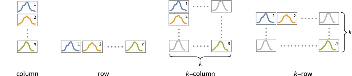
- Possible settings for PlotLayout that show single curves in multiple plot panels include:
-
"Column" use separate curves in a column of panels "Row" use separate curves in a row of panels {"Column",k},{"Row",k} use k columns or rows {"Column",UpTo[k]},{"Row",UpTo[k]} use at most k columns or rows - The arguments supplied to RegionFunction, MeshFunctions and ColorFunction are x and f, where f can be the PDF, CDF, etc. of the distribution.
- Possible highlighting effects for Highlighted and PlotHighlighting include:
-
style highlight the indicated curve 
"Ball" highlight and label the indicated point in a curve 
"Dropline" highlight and label the indicated point in a curve with drop lines to the axes 
"XSlice" highlight and label all points along a vertical slice 
"YSlice" highlight and label all points along a horizontal slice 
Placed[effect,pos] statically highlight the given position pos - Highlight position specifications pos include:
-
x,{x} effect at {x,y} with y chosen automatically {x,y} effect at {x,y} {pos1,pos2,…} multiple positions posi - With ScalingFunctions->{sx,sy}, the
 coordinate is scaled using sx, and the
  coordinate is scaled using sy.
Examples
open all close allBasic Examples (4)
Plot a smooth histogram of a set of dates:
Short[dates = EntityValue[EntityClass["Satellite", "GNSS"], "LaunchDate"], 5]SmoothDateHistogram[dates]Plot histograms for multiple datasets:
SmoothDateHistogram[{EntityValue[EntityClass["Satellite", "CommunicationMission"], "LaunchDate"], EntityValue[EntityClass["Satellite", "GNSS"], "LaunchDate"]}, PlotLegends -> {"communication", "navigation"}]Plot the CDF of the data instead of the PDF:
SmoothDateHistogram[{DateObject[{284, 7, 9}, "Day"], DateObject[{1778, 4, 30}, "Day"], DateObject[{1216, 8, 9}, "Day"], DateObject[{1093, 11, 12}, "Day"], DateObject[{1163, 10, 10}, "Day"], DateObject[{1255, 2, 10}, "Day"], DateObject[{1570, 8, 16}, "Day"], DateObject[{587, 10, 13}, "Day"], DateObject[{319, 11, 19}, "Day"], DateObject[{1295, 4, 20}, "Day"]}, Automatic, "CDF"]SmoothDateHistogram[EntityValue[EntityClass["Satellite", "GNSS"], "LaunchDate"], "Year"]Scope (21)
Data (5)
SmoothDateHistogram[{IconizedObject[«Earthquakes in USA since 2000»], IconizedObject[«Earthquakes in Mexico since 2000»], IconizedObject[«Earthquakes in Japan since 2000»]}]Create a smooth histogram from dates in an event series:
SmoothDateHistogram[EventSeries[{{DateObject[{2025, 2, 2}, "Day"], 1}, {DateObject[{2025, 2, 24}, "Day"], 2}, {DateObject[{2025, 3, 16}, "Day"], 3}, {DateObject[{2025, 5, 2}, "Day"], 4}}]]Create a smooth histogram from dates in an association:
SmoothDateHistogram[<|"event1" -> DateObject[{2025, 2, 2}, "Day"], "event2" -> DateObject[{2025, 2, 24}, "Day"], "event3" -> DateObject[{2025, 3, 16}, "Day"], "event4" -> DateObject[{2025, 5, 2}, "Day"]|>]Plot an association of datasets:
SmoothDateHistogram[<|"USA" -> IconizedObject[«Earthquakes in USA since 2000»], "Mexico" -> IconizedObject[«Earthquakes in Mexico since 2000»], "Japan" -> IconizedObject[«Earthquakes in Japan since 2000»]|>]SmoothDateHistogram[{IconizedObject[«Earthquakes in USA since 2000»], IconizedObject[«Earthquakes in Mexico since 2000»], IconizedObject[«Earthquakes in Japan since 2000»]}, PlotLayout -> "Stacked"]Tabular Data (1)
tabular = ResourceData["Sample Tabular Data: Sales Data"]Create a smooth date histogram for the sales dates:
SmoothDateHistogram[tabular -> "Date"]SmoothDateHistogram[tabular -> "Date", "Week"]Use PivotToColumns to generate columns of dates grouped by region:
tabular = PivotToColumns[tabular, "Region" -> "Date"]Create a smooth date histogram for sales in each region:
SmoothDateHistogram[tabular -> {"Midwest", "Northeast", "South", "West"}, PlotLegends -> {"Midwest", "Northeast", "South", "West"}]Bandwidth and Kernels (4)
By default, the height of the histogram displays the PDF of the date distribution:
SmoothDateHistogram[IconizedObject[«EarthQuakes in USA since 2000»], Automatic, "PDF", Filling -> Axis]Use the CDF as the height function:
SmoothDateHistogram[IconizedObject[«EarthQuakes in USA since 2000»], Automatic, "CDF", Filling -> Axis]Use the survival function as the height function:
SmoothDateHistogram[IconizedObject[«EarthQuakes in USA since 2000»], Automatic, "SF", Filling -> Axis]Use one year as the bandwidth for the smooth histogram:
SmoothDateHistogram[IconizedObject[«EarthQuakes in USA since 2000»], "Year"]SmoothDateHistogram[IconizedObject[«EarthQuakes in USA since 2000»], "Month"]SmoothDateHistogram[IconizedObject[«EarthQuakes in USA since 2000»], Quantity[6, "Months"]]Wrappers (3)
Use wrappers on individual datasets or collections of datasets:
SmoothDateHistogram[{IconizedObject[«Earthquakes in USA since 2000»], Style[IconizedObject[«Earthquakes in Mexico since 2000»], Red]}]SmoothDateHistogram[Style[{IconizedObject[«Earthquakes in USA since 2000»], IconizedObject[«Earthquakes in Mexico since 2000»]}, AbsoluteThickness[1]]]SmoothDateHistogram[Style[{IconizedObject[«Earthquakes in USA since 2000»], Style[IconizedObject[«Earthquakes in Mexico since 2000»], Red], IconizedObject[«Earthquakes in Japan since 2000»]}, AbsoluteThickness[1]]]Use PopupWindow to provide additional drilldown information:
SmoothDateHistogram[PopupWindow[IconizedObject[«Earthquakes in USA since 2000»], DateHistogram[IconizedObject[«Earthquakes in USA since 2000»], "Year", PlotLabel -> "Number of Earthquakes per year"]]]Button can be used to trigger any action:
SmoothDateHistogram[{Button[IconizedObject[«Earthquakes in USA since 2000»], Speak["US earthquakes in the last 25 years"]],
	Button[IconizedObject[«Earthquakes in Mexico since 2000»], Speak["Mexico earthquakes in the last 25 years"]]}]
Styling and Appearance (4)
Use an explicit list of styles for the lines:
SmoothDateHistogram[{IconizedObject[«Dates1»], IconizedObject[«Dates2»]}, PlotStyle -> {Red, Blue}]Style wrapper can be used to override styles:
SmoothDateHistogram[{IconizedObject[«Dates1»], Style[IconizedObject[«Dates2»], Red]}, PlotStyle -> Gray]SmoothDateHistogram[{IconizedObject[«Dates1»], IconizedObject[«Dates2»]}, PlotTheme -> "Monochrome"]Specify a range of interest for the plot:
SmoothDateHistogram[IconizedObject[«Earthquakes in USA since 2000»], Automatic, "PDF", PlotRange -> {{DateObject["2010"], DateObject["2030"]}, Automatic}]Labeling and Legending (4)
Use Labeled to add a label to a dataset:
data1 = EntityValue[EntityClass["Satellite", "CommunicationMission"], "LaunchDate"];
data2 = EntityValue[EntityClass["Satellite", "GNSS"], "LaunchDate"];
SmoothDateHistogram[{data1, Labeled[data2, "label", Above]}]data = EntityValue[EntityClass["Satellite", "GNSS"], "LaunchDate"];SmoothDateHistogram[Labeled[data, "label", Above]]SmoothDateHistogram[Labeled[data, "label", After]]Add categorical legend entries for datasets:
SmoothDateHistogram[{EntityValue[EntityClass["Satellite", "CommunicationMission"], "LaunchDate"], EntityValue[EntityClass["Satellite", "GNSS"], "LaunchDate"]}, PlotLegends -> {"communication", "navigation"}]Use Placed to affect the positioning of legends:
SmoothDateHistogram[{EntityValue[EntityClass["Satellite", "CommunicationMission"], "LaunchDate"], EntityValue[EntityClass["Satellite", "GNSS"], "LaunchDate"]}, PlotLegends -> Placed[{"communication", "navigation"}, Below]]Options (78)
Axes (4)
SmoothDateHistogram[IconizedObject[«data»]]Use AxesFalse to turn off axes:
SmoothDateHistogram[IconizedObject[«data»], Axes -> False]Use AxesOrigin to specify where the axes intersect:
SmoothDateHistogram[IconizedObject[«data»], Frame -> False, Axes -> True, AxesOrigin -> {"April 20,2010", 0}]Turn each axis on individually:
{SmoothDateHistogram[IconizedObject[«data»], Axes -> {True, False}], SmoothDateHistogram[IconizedObject[«data»], Axes -> {False, True}]}AxesLabel (3)
AxesOrigin (2)
AxesStyle (4)
Change the style for the axes:
SmoothDateHistogram[IconizedObject[«data»], Axes -> True, AxesStyle -> Red]Specify the style of each axis:
SmoothDateHistogram[IconizedObject[«data»], Axes -> True, AxesStyle -> {{Thick, Red}, {Thick, Blue}}]Use different styles for the ticks and the axes:
SmoothDateHistogram[IconizedObject[«data»], Axes -> True, AxesStyle -> Green, TicksStyle -> Red]Use different styles for the labels and the axes:
SmoothDateHistogram[IconizedObject[«data»], Axes -> True, AxesStyle -> Green, LabelStyle -> Red]ClippingStyle (4)
Omit clipped regions of the plot:
SmoothDateHistogram[{IconizedObject[«dates»], IconizedObject[«dates»] + Quantity[100, "Years"]}]Show the clipped regions as dashed sections:
SmoothDateHistogram[{IconizedObject[«dates»], IconizedObject[«dates»] + Quantity[100, "Years"]}, ClippingStyle -> Automatic]Show the clipped regions with red lines:
SmoothDateHistogram[{IconizedObject[«dates»], IconizedObject[«dates»] + Quantity[100, "Years"]}, ClippingStyle -> Red]Show the clipped regions as red and thick:
SmoothDateHistogram[{IconizedObject[«dates»], IconizedObject[«dates»] + Quantity[100, "Years"]}, ClippingStyle -> Directive[Red, Thick]]ColorFunction (5)
SmoothDateHistogram[EntityValue[EntityClass["Satellite", "GNSS"], "LaunchDate"], ColorFunction -> Function[{x, y}, Hue[x]]]SmoothDateHistogram[EntityValue[EntityClass["Satellite", "GNSS"], "LaunchDate"], ColorFunction -> Function[{x, y}, Hue[y]]]Color with a named color scheme:
SmoothDateHistogram[EntityValue[EntityClass["Satellite", "GNSS"], "LaunchDate"], ColorFunctionScaling -> True, ColorFunction -> "DarkRainbow"]Fill with the color used for the curve:
SmoothDateHistogram[EntityValue[EntityClass["Satellite", "GNSS"], "LaunchDate"], ColorFunctionScaling -> True, ColorFunction -> "DarkRainbow", Filling -> Axis]ColorFunction has higher priority than PlotStyle for coloring the curve:
SmoothDateHistogram[EntityValue[EntityClass["Satellite", "GNSS"], "LaunchDate"], ColorFunctionScaling -> True, ColorFunction -> "DarkRainbow", PlotStyle -> Directive[Red, Thick]]Use Automatic in MeshShading to use ColorFunction:
SmoothDateHistogram[EntityValue[EntityClass["Satellite", "GNSS"], "LaunchDate"], ColorFunctionScaling -> True, ColorFunction -> "DarkRainbow", PlotStyle -> Directive[Red, Thick], Mesh -> 9, MeshShading -> {Automatic, StandardGray}, MeshStyle -> None]ColorFunctionScaling (2)
Color the line based on scaled ![]() value:
value:
SmoothDateHistogram[EntityValue[EntityClass["Satellite", "GNSS"], "LaunchDate"], ColorFunction -> Function[{x, y}, Hue[y]], PlotStyle -> Thick, ColorFunctionScaling -> True]Color the line based on unscaled ![]() values:
values:
SmoothDateHistogram[EntityValue[EntityClass["Satellite", "GNSS"], "LaunchDate"], Automatic, "CHF", ColorFunction -> Function[{x, y}, If[y > 5, Red, Blue]], ColorFunctionScaling -> False]DateTicksFormat (1)
Use the last two digits of the year to label the date axis:
SmoothDateHistogram[EntityValue[EntityClass["Satellite", "GNSS"], "LaunchDate"], DateTicksFormat -> "YearShort"]Combine date elements with regular text elements:
SmoothDateHistogram[EntityValue[EntityClass["Satellite", "GNSS"], "LaunchDate"], DateTicksFormat -> {"`", "YearShort"}]Filling (5)
Use symbolic or explicit values:
Table[SmoothDateHistogram[EntityValue[EntityClass["Satellite", "GNSS"], "LaunchDate"], Filling -> c, PlotLabel -> c], {c, {Top, Bottom, Axis, N@Power[10, -9]}}]By default, overlapping fills combine using opacity:
SmoothDateHistogram[{IconizedObject[«dates»], IconizedObject[«dates»] + Quantity[100, "Years"]}, Filling -> Axis]Fill between curve 1 and the ![]() axis:
axis:
SmoothDateHistogram[{IconizedObject[«dates»], IconizedObject[«dates»] + Quantity[50, "Years"]}, Filling -> {1 -> Axis}]SmoothDateHistogram[{IconizedObject[«dates»], IconizedObject[«dates»] + Quantity[50, "Years"]}, Filling -> {1 -> {2}}]Fill between datasets using a particular style:
SmoothDateHistogram[{IconizedObject[«dates»], IconizedObject[«dates»] + Quantity[50, "Years"]}, Filling -> {1 -> {{2}, Directive[Orange, Opacity[.6]]}}]FillingStyle (3)
Fill below the curve with light gray:
SmoothDateHistogram[EntityValue[EntityClass["Satellite", "GNSS"], "LaunchDate"], Filling -> Bottom, FillingStyle -> LightGray]Hatch the area below the curve:
SmoothDateHistogram[EntityValue[EntityClass["Satellite", "GNSS"], "LaunchDate"], Filling -> Bottom, FillingStyle -> HatchFilling["Diagonal"]]SmoothDateHistogram[{IconizedObject[«dates»], IconizedObject[«dates»] + Quantity[25, "Years"]}, Filling -> Bottom, FillingStyle -> Directive[Opacity[0.5], Orange]]Use a variable filling style obtained from a ColorFunction:
SmoothDateHistogram[EntityValue[EntityClass["Satellite", "GNSS"], "LaunchDate"], ColorFunction -> Function[{x, y}, Hue[y]], Filling -> Axis, FillingStyle -> Automatic]ImageSize (7)
Use named sizes such as Tiny, Small, Medium and Large:
{SmoothDateHistogram[{...}, ImageSize -> Tiny], SmoothDateHistogram[{...}, ImageSize -> Small]}Specify the width of the plot:
{SmoothDateHistogram[{...}, ImageSize -> 150], SmoothDateHistogram[{...}, AspectRatio -> 1.5, ImageSize -> 150]}Allow the width and height to be up to a certain 200 points wide:
{SmoothDateHistogram[{...}, ImageSize -> UpTo[200]], SmoothDateHistogram[{...}, AspectRatio -> 2, ImageSize -> UpTo[200]]}Specify the width and height for a graphic, padding with space if necessary:
SmoothDateHistogram[{...}, ImageSize -> {200, 200}, Background -> StandardYellow]Setting AspectRatioFull will fill the available space:
SmoothDateHistogram[{...}, AspectRatio -> Full, ImageSize -> {200, 200}, Background -> StandardYellow]Use maximum sizes for the width and height:
{SmoothDateHistogram[{...}, ImageSize -> {UpTo[150], UpTo[100]}], SmoothDateHistogram[{...}, AspectRatio -> 2, ImageSize -> {UpTo[150], UpTo[100]}]}Use ImageSizeFull to fill the available space in an object:
Framed[Pane[SmoothDateHistogram[{...}, AspectRatio -> Full, ImageSize -> Full, Background -> StandardYellow], {200, 200}]]Specify the image size as a fraction of the available space:
Framed[Pane[SmoothDateHistogram[{...}, AspectRatio -> Full, ImageSize -> {Scaled[0.5], Scaled[0.5]}, Background -> StandardYellow], {200, 200}]]MeshFunctions (2)
Use a mesh evenly spaced in the ![]() and
and ![]() directions:
directions:
Table[SmoothDateHistogram[IconizedObject[«data»], MeshFunctions -> {Function[{x, y}, Evaluate[f]]}, Mesh -> 5, MeshStyle -> Directive[PointSize[Medium], Red], PlotLabel -> f], {f, {x, y}}]Show five mesh levels in the ![]() direction (red) and 10 in the
direction (red) and 10 in the ![]() direction (blue):
direction (blue):
SmoothDateHistogram[IconizedObject[«data»], Mesh -> {5, 10}, MeshFunctions -> {#1&, #2&}, MeshStyle -> {Directive[PointSize[Medium], Black], Directive[PointSize[Medium], Red]}]MeshShading (6)
Alternate red and blue segments of equal width in the ![]() direction:
direction:
SmoothDateHistogram[EntityValue[EntityClass["Satellite", "GNSS"], "LaunchDate"], "Year", Mesh -> 10, MeshShading -> {Red, Blue}]Use None to remove segments:
SmoothDateHistogram[EntityValue[EntityClass["Satellite", "GNSS"], "LaunchDate"], "Year", Mesh -> 10, MeshShading -> {Red, None}]MeshShading can be used with PlotStyle:
SmoothDateHistogram[EntityValue[EntityClass["Satellite", "GNSS"], "LaunchDate"], "Year", Mesh -> 10, PlotStyle -> Thick, MeshFunctions -> {#1&}, MeshShading -> {Red, Blue}]MeshShading has higher priority than PlotStyle for styling the curve:
SmoothDateHistogram[EntityValue[EntityClass["Satellite", "GNSS"], "LaunchDate"], "Year", Mesh -> 10, PlotStyle -> Thick, MeshFunctions -> {#1&}, PlotStyle -> Green, MeshShading -> {Red, Blue}]Use PlotStyle for some segments by setting MeshShading to Automatic:
SmoothDateHistogram[EntityValue[EntityClass["Satellite", "GNSS"], "LaunchDate"], "Year", Mesh -> 10, PlotStyle -> Directive[Thick, Yellow], MeshFunctions -> {#1&}, MeshShading -> {Red, Automatic}]MeshShading can be used with ColorFunction:
SmoothDateHistogram[EntityValue[EntityClass["Satellite", "GNSS"], "LaunchDate"], "Year", Mesh -> 10, PlotStyle -> Thick, MeshFunctions -> {#1&}, MeshShading -> {StandardGray, Automatic},
	ColorFunction -> Function[{x, y}, Hue[x]]]
MeshStyle (4)
Color the mesh the same color as the plot:
SmoothDateHistogram[IconizedObject[«data»], Mesh -> 5, MeshStyle -> Automatic]Use a red mesh in the ![]() direction:
direction:
SmoothDateHistogram[IconizedObject[«data»], Mesh -> 5, MeshStyle -> Directive[PointSize[Medium], Red]]Use a red mesh in the ![]() direction and a blue mesh in the
direction and a blue mesh in the ![]() direction:
direction:
SmoothDateHistogram[IconizedObject[«data»], Mesh -> 5, MeshStyle -> {Directive[PointSize[Medium], Red], Directive[PointSize[Medium], Blue]}, MeshFunctions -> {#1&, #2&}]Use big red mesh points in the ![]() direction:
direction:
SmoothDateHistogram[IconizedObject[«data»], Mesh -> 5, MeshStyle -> Directive[PointSize[Large], Red]]PerformanceGoal (2)
Generate a higher-quality plot:
AbsoluteTiming[SmoothDateHistogram[EntityValue[EntityClass["Satellite", "GNSS"], "LaunchDate"], PerformanceGoal -> "Quality", ImageSize -> Medium]]Emphasize performance, possibly at the cost of quality:
AbsoluteTiming[SmoothDateHistogram[EntityValue[EntityClass["Satellite", "GNSS"], "LaunchDate"], PerformanceGoal -> "Speed", ImageSize -> Medium]]PlotHighlighting (9)
Plots have interactive coordinate callouts with the default setting PlotHighlightingAutomatic:
SmoothDateHistogram[{IconizedObject[«Dates1»], IconizedObject[«Dates2»]}]Use PlotHighlightingNone to disable the highlighting for the entire plot:
SmoothDateHistogram[{IconizedObject[«Dates1»], IconizedObject[«Dates2»]}, PlotHighlighting -> None]Use Highlighted[…,None] to disable highlighting for a single curve:
SmoothDateHistogram[{IconizedObject[«Dates1»], Highlighted[IconizedObject[«Dates2»], None]}]Move the mouse over a curve to highlight it using arbitrary graphics directives:
SmoothDateHistogram[{IconizedObject[«Dates1»], IconizedObject[«Dates2»]}, PlotHighlighting -> Directive[Red, Dashed, DropShadowing[]]]Move the mouse over the curve to highlight it with a ball and label:
SmoothDateHistogram[{IconizedObject[«Dates1»], IconizedObject[«Dates2»]}, PlotHighlighting -> "Ball"]Use a ball and label to highlight a specific point on the curve:
SmoothDateHistogram[{Highlighted[IconizedObject[«Dates1»], Placed["Ball", DateObject["1rst September 2025"]]], IconizedObject[«Dates2»]}]Move the mouse over the curve to highlight it with a label and drop lines to the axes:
SmoothDateHistogram[IconizedObject[«Dates1»], PlotHighlighting -> "Dropline"]Use a ball and label to highlight a specific point on the curve:
SmoothDateHistogram[Highlighted[IconizedObject[«Dates1»], Placed["Dropline", DateObject["1rst August 2025"]]]]Move the mouse over the plot to highlight it with a slice showing ![]() values corresponding to the
values corresponding to the ![]() position:
position:
SmoothDateHistogram[{IconizedObject[«Dates1»], IconizedObject[«Dates2»]}, PlotHighlighting -> "XSlice"]Highlight the curves at a fixed ![]() value:
value:
SmoothDateHistogram[Highlighted[{IconizedObject[«Dates1»], IconizedObject[«Dates2»]}, Placed["XSlice", DateObject["15th May 2025"]]]]Move the mouse over the plot to highlight it with a slice showing ![]() values corresponding to the
values corresponding to the ![]() position:
position:
SmoothDateHistogram[{IconizedObject[«Dates1»], IconizedObject[«Dates2»]}, PlotHighlighting -> "YSlice"]Highlight the curves at a fixed ![]() value:
value:
SmoothDateHistogram[Highlighted[IconizedObject[«Dates2»], Placed["YSlice", 2Power[10, -8]]]]Use a component that shows the points on the curve closest to the ![]() position of the mouse cursor:
position of the mouse cursor:
SmoothDateHistogram[{IconizedObject[«Dates1»], IconizedObject[«Dates2»]}, PlotHighlighting -> "XNearestPoint"]Specify the style for the points:
SmoothDateHistogram[{IconizedObject[«Dates1»], IconizedObject[«Dates2»]}, PlotHighlighting -> {"XNearestPoint", <|"Style" -> Red|>}]Use a component that shows the coordinates on the curve closest to the mouse cursor:
SmoothDateHistogram[{IconizedObject[«Dates1»], IconizedObject[«Dates2»]}, PlotHighlighting -> "XYLabel"]Use Callout options to change the appearance of the label:
SmoothDateHistogram[{IconizedObject[«Dates1»], IconizedObject[«Dates2»]}, PlotHighlighting -> {"XYLabel", <|"Appearance" -> "Corners", "CalloutMarker" -> "Circle"|>}]Combine components to create a custom effect:
SmoothDateHistogram[IconizedObject[«Dates1»], PlotHighlighting -> {{"XNearestPoint", <|"Style" -> Red|>}, {"XYLabel", <|"Appearance" -> "Corners", "CalloutMarker" -> "Circle"|>}}]PlotPoints (1)
PlotRange (2)
PlotRange is automatically calculated:
SmoothDateHistogram[IconizedObject[«dates»]]SmoothDateHistogram[IconizedObject[«dates»], PlotRange -> All]SmoothDateHistogram[IconizedObject[«dates»], PlotRange -> {All, All}]SmoothHistogram automatically chooses the plotting domain:
SmoothDateHistogram[IconizedObject[«dates»]]Plot over the middle 70% of the data:
SmoothDateHistogram[IconizedObject[«dates»], PlotRange -> {Quantile[IconizedObject[«dates»], {0.15, 0.85}], All}]PlotRangePadding (5)
Use the default padding around the contents of the plot:
SmoothDateHistogram[EntityValue[EntityClass["Satellite", "GNSS"], "LaunchDate"], Axes -> None, Frame -> True, PlotRangePadding -> Automatic]Omit any padding around the contents:
SmoothDateHistogram[EntityValue[EntityClass["Satellite", "GNSS"], "LaunchDate"], Axes -> None, Frame -> True, PlotRangePadding -> None]SmoothDateHistogram[EntityValue[EntityClass["Satellite", "GNSS"], "LaunchDate"], Axes -> None, Frame -> True, PlotRangePadding -> Scaled[0.1]]Use no horizontal padding and the automatic vertical padding:
SmoothDateHistogram[EntityValue[EntityClass["Satellite", "GNSS"], "LaunchDate"], "Year", Axes -> None, Frame -> True, PlotRangePadding -> {None, Automatic}]Use the automatic padding on the left and right, no padding on the bottom and 10% on the top:
data = EntityValue[EntityClass["Satellite", "GNSS"], "LaunchDate"];SmoothDateHistogram[data, Axes -> None, Frame -> True, PlotRangePadding -> {{Automatic, Automatic}, {None, Scaled[0.2]}}]PlotStyle (7)
SmoothDateHistogram[IconizedObject[«data»], PlotStyle -> Purple]Use dashing to style the plot:
SmoothDateHistogram[IconizedObject[«data»], PlotStyle -> Dashed]SmoothDateHistogram[IconizedObject[«data»], PlotStyle -> AbsoluteThickness[5]]Use Directive to combine styles for a single curve:
SmoothDateHistogram[IconizedObject[«data»], PlotStyle -> Directive[Purple, Dashed, AbsoluteThickness[5]]]By default, different styles are chosen for multiple curves:
SmoothDateHistogram[{IconizedObject[«data»], IconizedObject[«data2»]}]Explicitly specify the style for different curves:
SmoothDateHistogram[{IconizedObject[«data»], IconizedObject[«data2»]}, PlotStyle -> {Red, Blue}]Use the association-based syntax to set a base style for all data:
SmoothDateHistogram[{IconizedObject[«data»], IconizedObject[«data2»]}, PlotStyle -> <|"Base" -> AbsoluteThickness[4]|>]Use a different style for each of the datasets:
SmoothDateHistogram[{IconizedObject[«data»], IconizedObject[«data2»]}, PlotStyle -> <|"Lists" -> {StandardCyan, StandardRed}|>]Provide an overall base style as well as styles for each dataset:
SmoothDateHistogram[{IconizedObject[«data»], IconizedObject[«data2»]}, PlotStyle -> <|"Base" -> AbsoluteThickness[4], "Lists" -> {StandardCyan, StandardRed}|>]PlotStyle can be combined with ColorFunction:
SmoothDateHistogram[IconizedObject[«data»], PlotStyle -> Thick, ColorFunction -> Function[{x, y}, Hue[y]]]PlotStyle can be combined with MeshShading:
SmoothDateHistogram[IconizedObject[«data»], PlotStyle -> Directive[Opacity[0.5], Thick], Mesh -> 10, MeshFunctions -> {#1&}, MeshShading -> {Red, Blue}]MeshStyle by default uses the same style as PlotStyle:
SmoothDateHistogram[IconizedObject[«data»], PlotStyle -> Red, Mesh -> All]Text
Wolfram Research (2025), SmoothDateHistogram, Wolfram Language function, https://reference.wolfram.com/language/ref/SmoothDateHistogram.html (updated 2026).
CMS
Wolfram Language. 2025. "SmoothDateHistogram." Wolfram Language & System Documentation Center. Wolfram Research. Last Modified 2026. https://reference.wolfram.com/language/ref/SmoothDateHistogram.html.
APA
Wolfram Language. (2025). SmoothDateHistogram. Wolfram Language & System Documentation Center. Retrieved from https://reference.wolfram.com/language/ref/SmoothDateHistogram.html