


LayeredGraphPlot
generates a layered plot of the graph g.
LayeredGraphPlot[{e1,e2,…}]
generates a layered plot of the graph with edges ej.
LayeredGraphPlot[{…,w[ei],…}]
plots ei with features defined by the symbolic wrapper w.
LayeredGraphPlot[{vi 1vj 1,…}]
uses rules vikvjk to specify the graph g.
uses the adjacency matrix m to specify the graph g.
LayeredGraphPlot[…,vpos]
places the dominant vertex v in the plot at position pos.
Details and Options
- LayeredGraphPlot attempts to place vertices in a series of "layers".
- LayeredGraphPlot supports the same vertices and edges as Graph.
- The following special wrappers can be used for the edges ei:
-
Annotation[ei,label] provide an annotation Button[ei,action] define an action to execute when the element is clicked EventHandler[ei,…] define a general event handler for the element Hyperlink[ei,uri] make the element act as a hyperlink Labeled[ei,…] display the element with labeling PopupWindow[ei,cont] attach a popup window to the element StatusArea[ei,label] display in the status area when the element is moused over Style[ei,opts] show the element using the specified styles Tooltip[ei,label] attach an arbitrary tooltip to the element - LayeredGraphPlot by default puts "dominant" vertices at the top, and puts vertices lower in the "hierarchy" progressively further down.
- LayeredGraphPlot[g,pos] places the dominant vertices at position pos.
- Possible positions pos are: Top, Bottom, Left, Right.
- By default, LayeredGraphPlot places each dominant vertex at the top.
- LayeredGraphPlot has the same options as Graphics, with the following additions and changes: [List of all options]
-
DataRange Automatic the range of vertex coordinates to generate DirectedEdges Automatic whether to interpret Rule as DirectedEdge EdgeLabels None labels and placements for edges EdgeLabelStyle Automatic style to use for edge labels EdgeShapeFunction Automatic generate graphic shapes for edges EdgeStyle Automatic styles for edges GraphHighlight {} vertices and edges to highlight GraphHighlightStyle Automatic style for highlight PerformanceGoal Automatic aspects of performance to try to optimize PlotStyle Automatic graphics directives to determine styles PlotTheme Automatic overall theme for the graph VertexCoordinates Automatic coordinates for vertices VertexLabels None labels and placements for vertices VertexLabelStyle Automatic style to use for vertex labels VertexShape Automatic graphic shape for vertices VertexShapeFunction Automatic generate graphic shapes for vertices VertexSize Automatic size of vertices VertexStyle Automatic styles for vertices - Possible settings for PlotTheme include common base themes:
-
"Business" a bright, modern look appropriate for business presentations or infographics "Detailed" identify data by employing labels and tooltips "Marketing" elegant, eye-catching design suitable for marketing needs "Minimal" simple graph "Monochrome" single-color design "Scientific" candid design useful for analyzing detailed data with labels and tooltips "Web" clean, bold design suitable for a consumer website or blog "Classic" historical design of graph to remain compatible with existing uses - Graph features themes affect plot of vertices and edges. Feature themes include:
-
"LargeGraph" large graph 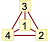
"ClassicLabeled" classic graph 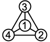
"IndexLabeled" index-labeled graph
List of all options
Examples
open all close allBasic Examples (5)
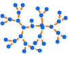
LayeredGraphPlot[PetersenGraph[]]Plot a graph specified by edge rules:
LayeredGraphPlot[{1 -> 2, 3 -> 1, 3 -> 2, 4 -> 1, 4 -> 2}]Plot a graph specified by its adjacency matrix:
LayeredGraphPlot[{{0, 1, 1, 1, 1}, {0, 0, 1, 1, 0}, {0, 0, 0, 0, 0}, {0, 0, 0, 0, 0}, {0, 0, 0, 0, 0}}]Drawing a graph with different orientation from the default:
LayeredGraphPlot[{1 -> 2, 1 -> 3, 2 -> 3, 1 -> 4, 2 -> 4, 1 -> 5}, Left]LayeredGraphPlot[{1 -> 2, 1 -> 3, 2 -> 3, 1 -> 4, 2 -> 4, 1 -> 5}, 2 -> Automatic, VertexLabels -> Automatic]Scope (9)
Graph Specification (4)
Specify a graph using a graph:
LayeredGraphPlot[Graph[{03, 05, 08, 010, 38}]]Specify a graph using a rule list:
LayeredGraphPlot[{0 -> 3, 0 -> 5, 0 -> 8, 0 -> 10, 3 -> 8}]Specify a graph using a dense adjacency matrix:
LayeredGraphPlot[{{0, 1, 1, 1, 1}, {0, 0, 0, 1, 0}, {0, 0, 0, 0, 0}, {0, 0, 0, 0, 0}, {0, 0, 0, 0, 0}}]Specify a graph using a sparse adjacency matrix:
LayeredGraphPlot[SparseArray[{{1, 2}, {1, 3}, {1, 4}, {1, 5}, {2, 4}} -> 1, {5, 5}]]Graph Styling (5)
LayeredGraphPlot[{1 -> 2, 1 -> 7, 1 -> 11, 2 -> 5, Labeled[1 -> 5, "1->5"]}]LayeredGraphPlot[{1 -> 2, 1 -> 7, 1 -> 11, 2 -> 5, 1 -> 5, 5 -> 5, 1 -> 5}, VertexLabels -> Automatic]LayeredGraphPlot[{1 -> 2, 1 -> 7, 1 -> 11, 2 -> 5, 1 -> 5}, DirectedEdges -> False]Plot a disconnected graph using different packing methods:
Table[Framed@LayeredGraphPlot[Table[i -> Mod[i ^ 2, 31], {i, 0, 31}], GraphLayout -> {"PackingLayout" -> pm}], {pm, {Automatic, "ClosestPacking"}}]Draw with different orientations:
Row@Table[LayeredGraphPlot[{1 -> 3, 1 -> 4, 1 -> 5, 3 -> 5, 3 -> 6}, pos, PlotLabel -> pos], {pos, {Left, Top, Right, Bottom}}]Options (50)
AspectRatio (4)
By default, the ratio of the height to width for the plot is determined automatically:
LayeredGraphPlot[{1 -> 2, 1 -> 3, 2 -> 3, 1 -> 4, 2 -> 4}]Make the height the same as the width with AspectRatio1:
LayeredGraphPlot[{1 -> 2, 1 -> 3, 2 -> 3, 1 -> 4, 2 -> 4}, AspectRatio -> 1]Use numerical value to specify the height-to-width ratio:
LayeredGraphPlot[{1 -> 2, 1 -> 3, 2 -> 3, 1 -> 4, 2 -> 4}, AspectRatio -> 1 / 2]AspectRatioFull adjusts the height and width to tightly fit inside other constructs:
plot = LayeredGraphPlot[{1 -> 2, 1 -> 3, 2 -> 3, 1 -> 4, 2 -> 4}, AspectRatio -> Full];{Framed[Pane[plot, {100, 150}]], Framed[Pane[plot, {100, 100}]]}Axes (3)
By default, Axes are not drawn for LayeredGraphPlot:
LayeredGraphPlot[{1 -> 2, 1 -> 3, 2 -> 3, 1 -> 4, 2 -> 4}]Use AxesTrue to turn on axes:
LayeredGraphPlot[{1 -> 2, 1 -> 3, 2 -> 3, 1 -> 4, 2 -> 4}, Axes -> True]Turn each axis on individually:
{LayeredGraphPlot[{1 -> 2, 1 -> 3, 2 -> 3, 1 -> 4, 2 -> 4}, Axes -> {True, False}], LayeredGraphPlot[{1 -> 2, 1 -> 3, 2 -> 3, 1 -> 4, 2 -> 4}, Axes -> {False, True}]}AxesLabel (3)
No axes labels are drawn by default:
LayeredGraphPlot[{1 -> 2, 1 -> 3, 2 -> 3, 1 -> 4, 2 -> 4}, Axes -> True]LayeredGraphPlot[{1 -> 2, 1 -> 3, 2 -> 3, 1 -> 4, 2 -> 4}, Axes -> True, AxesLabel -> y]LayeredGraphPlot[{1 -> 2, 1 -> 3, 2 -> 3, 1 -> 4, 2 -> 4}, Axes -> True, AxesLabel -> {x, y}]AxesOrigin (2)
The position of the axes is determined automatically:
LayeredGraphPlot[{1 -> 2, 1 -> 3, 2 -> 3, 1 -> 4, 2 -> 4}, Axes -> True]Specify an explicit origin for the axes:
LayeredGraphPlot[{1 -> 2, 1 -> 3, 2 -> 3, 1 -> 4, 2 -> 4}, Axes -> True, AxesOrigin -> {2, 0}]AxesStyle (4)
Change the style for the axes:
LayeredGraphPlot[{1 -> 2, 1 -> 3, 2 -> 3, 1 -> 4, 2 -> 4}, Axes -> True, AxesStyle -> Red]Specify the style of each axis:
LayeredGraphPlot[{1 -> 2, 1 -> 3, 2 -> 3, 1 -> 4, 2 -> 4}, Axes -> True, AxesStyle -> {{Thick, Brown}, {Thick, Blue}}]Use different styles for the ticks and the axes:
LayeredGraphPlot[{1 -> 2, 1 -> 3, 2 -> 3, 1 -> 4, 2 -> 4}, Axes -> True, AxesStyle -> Green, TicksStyle -> Red]Use different styles for the labels and the axes:
LayeredGraphPlot[{1 -> 2, 1 -> 3, 2 -> 3, 1 -> 4, 2 -> 4}, Axes -> True, AxesStyle -> Green, LabelStyle -> Red]DataRange (1)
DirectedEdges (2)
Frame (4)
LayeredGraphPlot does not use a frame by default:
LayeredGraphPlot[{1 -> 2, 2 -> 3, 3 -> 4, 1 -> 4, 1 -> 3}]Use FrameTrue to draw a frame around the plot:
LayeredGraphPlot[{1 -> 2, 2 -> 3, 3 -> 4, 1 -> 4, 1 -> 3}, Frame -> True]Draw a frame on the left and right edges:
LayeredGraphPlot[{1 -> 2, 2 -> 3, 3 -> 4, 1 -> 4, 1 -> 3}, Frame -> {{True, True}, {False, False}}]Draw a frame on the left and bottom edges:
LayeredGraphPlot[{1 -> 2, 2 -> 3, 3 -> 4, 1 -> 4, 1 -> 3}, Frame -> {{True, False}, {True, False}}]FrameLabel (4)
Place a label along the bottom frame of a plot:
LayeredGraphPlot[{1 -> 2, 2 -> 3, 3 -> 4, 1 -> 4, 1 -> 3}, Frame -> True, FrameLabel -> {"label"}]Frame labels are placed on the bottom and left frame edges by default:
LayeredGraphPlot[{1 -> 2, 2 -> 3, 3 -> 4, 1 -> 4, 1 -> 3}, Frame -> True, FrameLabel -> {"bottom", "left"}]Place labels on each of the edges in the frame:
LayeredGraphPlot[{1 -> 2, 2 -> 3, 3 -> 4, 1 -> 4, 1 -> 3}, Frame -> True, FrameLabel -> {{"left", "right"}, {"bottom", "top"}}]Use a customized style for both labels and frame tick labels:
LayeredGraphPlot[{1 -> 2, 2 -> 3, 3 -> 4, 1 -> 4, 1 -> 3}, Frame -> True, FrameLabel -> {{"left", "right"}, {"bottom", "top"}}, LabelStyle -> Directive[Bold, StandardGray]]FrameStyle (2)
Specify the style of the frame:
LayeredGraphPlot[{1 -> 2, 2 -> 3, 3 -> 4, 1 -> 4, 1 -> 3}, Frame -> True, FrameStyle -> Directive[StandardGray, Thick]]Specify the style for each frame edge:
LayeredGraphPlot[{1 -> 2, 2 -> 3, 3 -> 4, 1 -> 4, 1 -> 3}, Frame -> True, FrameStyle -> {{Directive[Green, Thick], Red}, {Directive[Gray, Thick], Blue}}]FrameTicks (8)
Frame ticks are not placed automatically by default:
LayeredGraphPlot[{1 -> 2, 2 -> 3, 3 -> 4, 1 -> 4, 1 -> 3}, Frame -> True]LayeredGraphPlot[{1 -> 2, 2 -> 3, 3 -> 4, 1 -> 4, 1 -> 3}, Frame -> True, FrameTicks -> True]Use frame ticks on the bottom edge:
LayeredGraphPlot[{1 -> 2, 2 -> 3, 3 -> 4, 1 -> 4, 1 -> 3}, Frame -> True, FrameTicks -> {{None, None}, {True, None}}]Use All to include tick labels on all edges:
LayeredGraphPlot[{1 -> 2, 2 -> 3, 3 -> 4, 1 -> 4, 1 -> 3}, Frame -> True, FrameTicks -> All]Place tick marks at specific positions:
LayeredGraphPlot[{1 -> 2, 2 -> 3, 3 -> 4, 1 -> 4, 1 -> 3}, Frame -> True, FrameTicks -> {{{0.2, 0.4}, None}, {{0.5, 1.0}, None}}]Draw frame tick marks at the specified positions with specific labels:
LayeredGraphPlot[{1 -> 2, 2 -> 3, 3 -> 4, 1 -> 4, 1 -> 3}, Frame -> True, FrameTicks -> {{{{0.2, a}, {0.4, b}}, None}, {{{0.5, c}, {1.0, d}}, None}}]Specify the lengths for tick marks as a fraction of the graphics size:
LayeredGraphPlot[{1 -> 2, 2 -> 3, 3 -> 4, 1 -> 4, 1 -> 3}, Frame -> True, FrameTicks -> {{{{0.2, a, .1}, {0.4, b, .1}}, None}, {{{0.5, c, .1}, {1.0, d, .1}}, None}}]Use different sizes in the positive and negative directions for each tick mark:
LayeredGraphPlot[{1 -> 2, 2 -> 3, 3 -> 4, 1 -> 4, 1 -> 3}, Frame -> True, FrameTicks -> {{None, None}, {{{0.5, a, {.1, .1}}, {1, b, {.1, .05}}}, None}}]Specify a style for each frame tick:
LayeredGraphPlot[{1 -> 2, 2 -> 3, 3 -> 4, 1 -> 4, 1 -> 3}, Frame -> True, FrameTicks -> {{None, None}, {{{0.3, a, {.4, .1}, Directive[Red, Thick, Dashed]}, {.5, b, {.25, .05}, Directive[Green, Thick, Dashed]}}, None}}]FrameTicksStyle (3)
By default, the frame ticks and frame tick labels use the same styles as the frame:
LayeredGraphPlot[{1 -> 2, 2 -> 3, 3 -> 4, 1 -> 4, 1 -> 3}, Frame -> True, FrameTicks -> True, FrameStyle -> Directive[Red]]Specify an overall style for the ticks, including the labels:
LayeredGraphPlot[{1 -> 2, 2 -> 3, 3 -> 4, 1 -> 4, 1 -> 3}, Frame -> True, FrameTicks -> True, FrameStyle -> Directive[Red], FrameTicksStyle -> Directive[Blue, Thick]]Use different style for the different frame edges:
LayeredGraphPlot[{1 -> 2, 2 -> 3, 3 -> 4, 1 -> 4, 1 -> 3}, Frame -> True, FrameTicks -> All, FrameTicksStyle -> {{Directive[Orange, Thick], Blue}, {Red, Green}}]ImageSize (7)
Use named sizes such as Tiny, Small, Medium and Large:
{LayeredGraphPlot[{1 -> 2, 1 -> 3, 2 -> 3, 1 -> 4, 2 -> 4}, ImageSize -> Tiny], LayeredGraphPlot[{1 -> 2, 1 -> 3, 2 -> 3, 1 -> 4, 2 -> 4}, ImageSize -> Small]}Specify the width of the plot:
{LayeredGraphPlot[{1 -> 2, 1 -> 3, 2 -> 3, 1 -> 4, 2 -> 4}, ImageSize -> 150], LayeredGraphPlot[{1 -> 2, 1 -> 3, 2 -> 3, 1 -> 4, 2 -> 4}, AspectRatio -> 1.5, ImageSize -> 150]}Specify the height of the plot:
{LayeredGraphPlot[{1 -> 2, 1 -> 3, 2 -> 3, 1 -> 4, 2 -> 4}, ImageSize -> {Automatic, 150}], LayeredGraphPlot[{1 -> 2, 1 -> 3, 2 -> 3, 1 -> 4, 2 -> 4}, AspectRatio -> 2, ImageSize -> {Automatic, 150}]}Allow the width and height to be up to a certain size:
{LayeredGraphPlot[{1 -> 2, 1 -> 3, 2 -> 3, 1 -> 4, 2 -> 4}, ImageSize -> UpTo[200]], LayeredGraphPlot[{1 -> 2, 1 -> 3, 2 -> 3, 1 -> 4, 2 -> 4}, AspectRatio -> 2, ImageSize -> UpTo[200]]}Specify the width and height for a graphic, padding with space if necessary:
LayeredGraphPlot[{1 -> 2, 1 -> 3, 2 -> 3, 1 -> 4, 2 -> 4}, ImageSize -> {200, 300}, Background -> LightBlue]Setting AspectRatioFull will fill the available space:
LayeredGraphPlot[{1 -> 2, 1 -> 3, 2 -> 3, 1 -> 4, 2 -> 4}, AspectRatio -> Full, ImageSize -> {200, 300}, Background -> LightBlue]Use maximum sizes for the width and height:
{LayeredGraphPlot[{1 -> 2, 1 -> 3, 2 -> 3, 1 -> 4, 2 -> 4}, ImageSize -> {UpTo[150], UpTo[100]}], LayeredGraphPlot[{1 -> 2, 1 -> 3, 2 -> 3, 1 -> 4, 2 -> 4}, AspectRatio -> 2, ImageSize -> {UpTo[150], UpTo[100]}]}Use ImageSizeFull to fill the available space in an object:
Framed[Pane[LayeredGraphPlot[{1 -> 2, 1 -> 3, 2 -> 3, 1 -> 4, 2 -> 4}, ImageSize -> Full, Background -> LightBlue], {200, 100}]]Specify the image size as a fraction of the available space:
Framed[Pane[LayeredGraphPlot[{1 -> 2, 1 -> 3, 2 -> 3, 1 -> 4, 2 -> 4}, ImageSize -> {Scaled[0.5], Scaled[0.5]}, Background -> LightBlue], {200, 100}]]PlotStyle (3)
Specify an overall style for the graph:
Table[LayeredGraphPlot[{1 -> 4, 1 -> 9, 4 -> 5, 0 -> 5, 3 -> 5, 3 -> 8, 3 -> 9}, PlotStyle -> ps], {ps, {Red, Dashed, Directive[Red, Dashed]}}]PlotStyle can be combined with VertexShapeFunction, which has higher priority:
LayeredGraphPlot[{1 -> 4, 1 -> 9, 4 -> 5, 0 -> 5, 3 -> 5, 3 -> 8, 3 -> 9}, PlotStyle -> Directive[PointSize[Large], Red], VertexShapeFunction -> Function[{p, l}, {Green, Point[p]}]]PlotStyle can be combined with EdgeShapeFunction, which has higher priority:
LayeredGraphPlot[{1 -> 4, 1 -> 9, 4 -> 5, 0 -> 5, 3 -> 5, 3 -> 8, 3 -> 9}, PlotStyle -> Directive[Dashed, Red], EdgeShapeFunction -> Function[{p, vl}, {Green, Line[p]}]]Applications (5)
LayeredGraphPlot[{"John" -> "plants", "lion" -> "John", "tiger" -> "John", "tiger" -> "deer", "lion" -> "deer", "deer" -> "plants", "mosquito" -> "lion", "frog" -> "mosquito", "mosquito" -> "tiger", "John" -> "cow", "cow" -> "plants", "mosquito" -> "deer", "mosquito" -> "John", "snake" -> "frog", "vulture" -> "snake"}, Left, PlotTheme -> "DiagramGreen"]A chart showing the relationships between shapes:
LayeredGraphPlot[{"Square" -> "Rectangle", "Rectangle" -> "Parallelogram", "Parallelogram" -> "Four-Sided Polygon", "Trapezoid" -> "Four-Sided Polygon", "Rectangle" -> "Trapezoid", "Four-Sided Polygon" -> "Polygon", "Polygon" -> "Shape", "Circle" -> "Ellipsoid", "Ellipsoid" -> "Shape", "Triangle" -> "Polygon", "Equilateral Triangle" -> "Isosceles Triangle", "Isosceles Triangle" -> "Triangle"}, PlotTheme -> "DiagramBlue", VertexSize -> {.4, .15}, AspectRatio -> 1.5]A flow chart for a computer program:
LayeredGraphPlot[{"Total" -> "TotalDispatch", "TotalList" -> "CheckThreading", "TotalList" -> "TotalDispatch", "TotalSparse" -> "TotalDispatch", "TotalSparse" -> "TotalDispatch", "TotalDispatch" -> "TotalDispatch", "TotalDispatch" -> "TotalList", "TotalDispatch" -> "TotalPacked", "TotalDispatch" -> "TotalSparse"}, PlotTheme -> "DiagramBlue", VertexSize -> {.4, .15}]A visual representation of a straight-line program, used for common subexpression elimination:
f[x_] := Module[{e1, e2, e3}, e1 = x + 1;e2 = Exp[x e1] + 1; e3 = e1 + Sin[x e2]; x + e3 + e1]LayeredGraphPlot[{x -> f, e3 -> f, e1 -> f, e1 -> e3, x -> e3, e2 -> e3, x -> e2, e1 -> e2, x -> e1}, PlotTheme -> "ClassicDiagram"]The relationships between early versions of the Unix operating system:
g = {"5th Edition" -> "6th Edition", "5th Edition" -> "PWB 1.0", "6th Edition" -> "1 BSD", "6th Edition" -> "Interdata", "6th Edition" -> "LSX", "6th Edition" -> "Mini Unix", "6th Edition" -> "Wollongong", "PWB 1.0" -> "PWB 1.2", "PWB 1.0" -> "USG 1.0", "1 BSD" -> "2 BSD", "Interdata" -> "PWB 2.0", "Interdata" -> "Unix/TS 3.0", "Interdata" -> "7th Edition", "PWB 1.2" -> "PWB 2.0", "USG 1.0" -> "USG 2.0", "USG 1.0" -> "CB Unix 1", "7th Edition" -> "2 BSD", "7th Edition" -> "32V", "7th Edition" -> "Xenix", "7th Edition" -> "Ultrix-11", "7th Edition" -> "UniPlus+", "7th Edition" -> "V7M", "PWB 2.0" -> "Unix/TS 3.0", "USG 2.0" -> "USG 3.0", "CB Unix 1" -> "CB Unix 2", "32V" -> "3 BSD", "Unix/TS 1.0" -> "Unix/TS 3.0", "USG 3.0" -> "Unix/TS 3.0", "CB Unix 2" -> "CB Unix 3", "3 BSD" -> "4 BSD", "V7M" -> "Ultrix-11", "Unix/TS 3.0" -> "TS 4.0", "CB Unix 3" -> "Unix/TS++", "CB Unix 3" -> "PDP-11 Sys V", "4 BSD" -> "4.1 BSD", "Unix/TS++" -> "TS 4.0", "4.1 BSD" -> "8th Edition", "4.1 BSD" -> "4.2 BSD", "4.1 BSD" -> "2.8 BSD", "2 BSD" -> "2.8 BSD", "TS 4.0" -> "System V.0", "4.2 BSD" -> "4.3 BSD", "4.2 BSD" -> "Ultrix-32", "2.8 BSD" -> "2.9 BSD", "2.8 BSD" -> "Ultrix-11", "System V.0" -> "System V.2", "8th Edition" -> "9th Edition", "System V.2" -> "System V.3"};LayeredGraphPlot[g, PlotTheme -> "ClassicDiagram", VertexSize -> {.5, .1}]Properties & Relations (3)
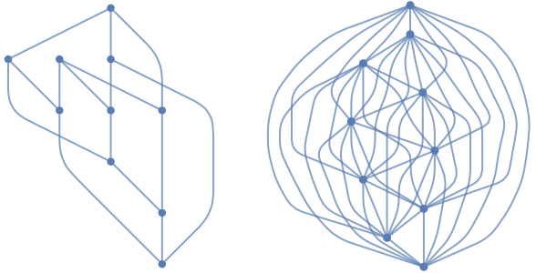
TreePlot provides a layered layout ignoring the direction of edges:
{TreePlot[{1 -> 4, 1 -> 6, 1 -> 8, 2 -> 6, 3 -> 8, 4 -> 5, 7 -> 8, 1 -> 7}, DirectedEdges -> True, VertexLabels -> "Name"], LayeredGraphPlot[{1 -> 4, 1 -> 6, 1 -> 8, 2 -> 6, 3 -> 8, 4 -> 5, 7 -> 8, 1 -> 7}, DirectedEdges -> True, VertexLabels -> "Name"]}Use GraphPlot or GraphPlot3D for general undirected graph drawing:
g = {1 -> 2, 1 -> 6, 1 -> 20, 2 -> 3, 2 -> 17, 3 -> 4, 3 -> 12, 4 -> 5, 4 -> 15, 5 -> 6, 5 -> 10, 6 -> 7, 7 -> 8, 7 -> 16, 8 -> 9, 8 -> 19, 9 -> 10, 9 -> 14, 10 -> 11, 11 -> 12, 11 -> 20, 12 -> 13, 13 -> 14, 13 -> 18, 14 -> 15, 15 -> 16, 16 -> 17, 17 -> 18, 18 -> 19, 19 -> 20};{GraphPlot[g], GraphPlot3D[g]}Use ArrayPlot or MatrixPlot to display matrices:
g = ExampleData[{"Matrix", "Bai/bfwa62"}, "Matrix"]{ArrayPlot[g], MatrixPlot[g]}Possible Issues (1)
When vertex coordinates are specified, all edges are shown as straight lines:
LayeredGraphPlot[{1 -> 2, 2 -> 3, 3 -> 4, 1 -> 4}, VertexLabels -> "Name", VertexCoordinates -> {{0, 2}, {0, 1}, {0, 0}, {2, -1}}]If explicit vertex coordinates are not specified, curved edges will be used:
LayeredGraphPlot[{1 -> 2, 2 -> 3, 3 -> 4, 1 -> 4}, VertexLabels -> "Name"]Neat Examples (1)
DaughterNuclides[s_List] := DeleteCases[Union[Apply[Join, Map[IsotopeData[#, "DaughterNuclides"]&, DeleteCases[s, _Missing]]]], _Missing]ReachableNuclides[s_List] := FixedPoint[Union[Join[#, DaughterNuclides[#]]]&, s]DecayNetwork[iso_List] :=
Apply[Join, Map[Thread[# -> DaughterNuclides[{#}]]&, ReachableNuclides[iso]]]DecayNetworkPlot[s_] := LayeredGraphPlot[Map[IsotopeData[#, "Symbol"]&, DecayNetwork[{s}], {2}], PerformanceGoal -> "Quality", VertexShapeFunction -> (Text[Framed[Style[#2, 8, Black], Background -> LightYellow], #1]&)]DecayNetworkPlot["Uranium235"]DecayNetworkPlot["Polonium189"]DecayNetworkPlot["Plutonium239"]Text
Wolfram Research (2007), LayeredGraphPlot, Wolfram Language function, https://reference.wolfram.com/language/ref/LayeredGraphPlot.html (updated 2020).
CMS
Wolfram Language. 2007. "LayeredGraphPlot." Wolfram Language & System Documentation Center. Wolfram Research. Last Modified 2020. https://reference.wolfram.com/language/ref/LayeredGraphPlot.html.
APA
Wolfram Language. (2007). LayeredGraphPlot. Wolfram Language & System Documentation Center. Retrieved from https://reference.wolfram.com/language/ref/LayeredGraphPlot.html