


PairwiseListPlot
PairwiseListPlot[{{y11,…,y1n},…,{ym1,…,ymn}}]
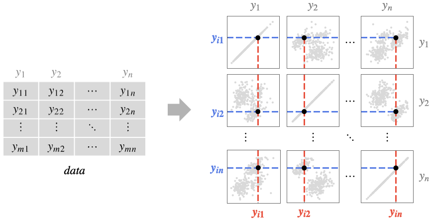
creates an array of scatter plots by plotting the data columns against each other in pairs.
PairwiseListPlot[{data1,data2,…}]
plots multiple sets of data in each plot panel.
Details and Options
- PairwiseListPlot is also known as a scatterplot array or matrix.
- It plots high-dimensional data by creating a grid of individual plots of just two data columns at a time.
- The plot compares column yi={y1i,y2i,…,ymi} against column yj={y1j,y2j,…,ymj} by plotting the points {ykj,yki} in panel {i,j}.
- The panel at row
 and column
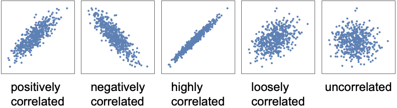
  shows how the data columns yi and yj relate to each other. There are different types of features of the data that can be identified from those panels. Once the feature has been identified it can also be quantified by further analysis of the data.
 - Correlation and covariance are measures of dependence between variables:
- Use Correlation and Covariance to do detailed analysis of correlation.
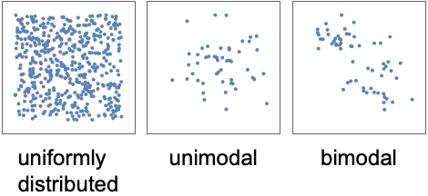
- The density of points is a measure of the number of points per unit area. The panels in PairwiseListPlot effectively show the two-dimensional marginal densities:
- Use PairwiseDensityHistogram and PairwiseSmoothDensityHistogram to more directly visualize the densities.
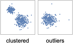
- Clusters are groups of similar points, indicating categories:
- Use FindClusters and ClusterClassify to do further analysis of these.
- Data values yij can be given in the following forms:
-
yij a real-valued number Quantity[yiji,unit] a quantity with a unit - Values that are not of the form above are taken to be missing and are not shown.
- PairwiseListPlot[Dataset[…]] plots the data from the dataset, using column labels to label the plot if available.
- PairwiseListPlot[Tabular[…]cspec] extracts and plots values from the tabular object using the column specification cspec.
- The following forms of column specifications cspec are allowed for plotting tabular data:
-
{coly1,…,colyn} plot the colyi against colyj in a pairwise manner - PairwiseListPlot takes the same options as Graphics, with the following changes and additions: [List of all options]
-
AspectRatio 1 ratio of height to width for each panel Background None background to use for each plot Frame Automatic whether to draw frames around each panel FrameTicks Automatic whether to label frame edges with ticks and labels GridLines Automatic whether to include gridlines in panels GridLinesStyle Automatic style for gridlines HeaderAlignment Center horizontal and vertical alignments of headers HeaderBackground Automatic background colors to use for headers HeaderDisplayFunction Automatic function to use to format headers Headers Automatic labels to use for each data column yi HeaderStyle None styles to use for headers PerformanceGoal $PerformanceGoal aspects of performance to try to optimize PlotFit None how to fit a curve to the points PlotFitElements Automatic fitted elements to show in the plot PlotHighlighting Automatic highlighting effect for points PlotInteractivity $PlotInteractivity whether to allow interactive elements PlotLayout Automatic how to arrange the panels PlotLegends Automatic legends for data PlotMarkers None markers to use to indicate each point PlotStyle Automatic graphics directives to determine styles of points PlotTheme $PlotTheme overall theme for the plot Spacings Automatic horizontal and vertical spacings - PlotLayout can have the following settings:
-

"Descending" data columns going down and to the right 
"Ascending" data columns going up and to the right 
"DescendingHalfMatrix" lower half of the descending layout 
"AscendingHalfMatrix" upper half of the ascending layout - Headers specifies the labels to use for each column in the data, and will generally be displayed above each column and after each row in the final plot.
- Possible settings include:
-
None leave the plot columns and rows unlabeled Automatic automatically label columns and rows All always include column and row labels "Indexed" number the columns and rows 1, 2, …, n {lbl1,lbl2,…,lbln} use the given labels lbli - HeaderAlignment determines how data column labels are aligned with regard to the plot columns and rows.
- HeaderAlignment can take the following forms:
-
Center center the labels in the header positions {h,v} separate horizontal and vertical alignments within the header position {cols,rows} use col for plot columns and row for plot rows - HeaderBackground and HeaderStyle can take the following forms:
-
None use ambient styling sty use the style sty for all headers {sty1,sty2,…,styn} use the given styles styifor successive headers {cols,rows} use col for plot columns and row for plot rows - HeaderDisplayFunction determines how headers are displayed.
- Possible settings are:
-
Automatic automatic formatting None use unprocessed labels - ColorData["DefaultPlotColors"] gives the default sequence of colors used by PlotStyle.
- The arguments to ColorFunction are yi1,yi2,…,yin. By default, the color function arguments are scaled per data column to be between 0 and 1.
- Use ColorFunctionScalingNone to use unscaled values, or ColorFunctionScaling{cfsc1,cfsc2,…} to selectively scale column values.
- Possible settings for PlotHighlighting include:
-
Automatic automatically highlight positions in the panels None disable interactive highlighting
List of all options
Examples
open all close allBasic Examples (4)
Create a pairwise plot of the columns against each other:
PairwiseListPlot[IconizedObject[«medical data»]]PairwiseListPlot[{IconizedObject[«4-cylinder autos»], IconizedObject[«6-cylinder autos»], IconizedObject[«8-cylinder autos»]}]Provide header names for the data:
PairwiseListPlot[IconizedObject[«iris data»], Headers -> {"sepal length", "sepal width", "petal length", "petal width"}]PairwiseListPlot[IconizedObject[«iris groups»], Headers -> {"petal length", "petal width", "sepal length", "sepal width"}]Scope (1)
Tabular Data (1)
iris = ResourceData["Sample Tabular Data: Fisher Iris"]Create a pairwise array of scatter plots:
PairwiseListPlot[iris -> {"SepalLength", "SepalWidth", "PetalLength", "PetalWidth"}]Use a different theme for the plot:
PairwiseListPlot[iris -> {"SepalLength", "SepalWidth", "PetalLength", "PetalWidth"}, PlotTheme -> "Marketing"]Options (56)
AspectRatio (2)
By default, PairwiseListPlot uses an equal height-to-width ratio:
PairwiseListPlot[IconizedObject[«iris data»]]Use a fixed height-to-width ratio:
PairwiseListPlot[IconizedObject[«iris data»], AspectRatio -> 1 / 2]Axes (3)
By default, Frame is used instead of Axes:
PairwiseListPlot[IconizedObject[«iris data»]]Use AxesTrue to turn on axes:
PairwiseListPlot[IconizedObject[«iris data»], Frame -> False, Axes -> True]Turn each axis on independently:
{PairwiseListPlot[IconizedObject[«iris data»], Frame -> False, Axes -> {True, False}], PairwiseListPlot[IconizedObject[«iris data»], Frame -> False, Axes -> {False, True}]}AxesStyle (4)
Change the style for the axes:
PairwiseListPlot[IconizedObject[«iris data»], ImageSize -> Medium, Frame -> False, Axes -> True, AxesStyle -> Red]Specify the style of each axis:
PairwiseListPlot[IconizedObject[«iris data»], ImageSize -> Medium, Frame -> False, Axes -> True, AxesStyle -> {Directive[Thick, Red], Directive[Thick, Blue]}]Use different styles for the ticks and the axes:
PairwiseListPlot[IconizedObject[«iris data»], ImageSize -> Medium, Frame -> False, Axes -> True, AxesStyle -> Green, TicksStyle -> Magenta]Use different styles for the labels and the axes:
PairwiseListPlot[IconizedObject[«iris data»], ImageSize -> Medium, Frame -> False, Axes -> True, AxesStyle -> Green, LabelStyle -> StandardGray]Background (2)
By default, PairwiseListPlot has a white background:
PairwiseListPlot[IconizedObject[«iris data»]]PairwiseListPlot[IconizedObject[«iris data»], Background -> GrayLevel[.9]]ColorFunction (3)
Color by scaled ![]() and
and ![]() coordinates:
coordinates:
Table[PairwiseListPlot[IconizedObject[«iris data»], ImageSize -> Small, ColorFunction -> f, PlotLabel -> f[x, y]], {f, {Hue[#]&, Hue[#2]&}}]Color with a named color scheme:
PairwiseListPlot[IconizedObject[«iris data»], ImageSize -> Medium, ColorFunction -> "DarkRainbow"]ColorFunction has higher priority than PlotStyle for coloring:
PairwiseListPlot[IconizedObject[«iris data»], ImageSize -> Medium, ColorFunction -> "DarkRainbow", PlotStyle -> Directive[Red, Thick]]Frame (2)
FrameStyle (1)
GridLines (2)
By default, PairwiseListPlot does not draw gridlines:
PairwiseListPlot[IconizedObject[«iris data»]]PairwiseListPlot[IconizedObject[«iris data»], GridLines -> Automatic, Background -> LightGray]HeaderBackground (1)
Headers (2)
Number the columns for unlabeled data:
PairwiseListPlot[{{0, 6, 9}, {4, 5, 8}, {0, 0, 5}, {4, 2, 9}, {9, 7, 6}, {10, 5, 6}, {0, 8, 4}, {8, 6, 10}, {10, 4, 0}, {9, 8, 1}}, Headers -> "Indexed"]Provide header names for the columns:
PairwiseListPlot[{{0, 6, 9}, {4, 5, 8}, {0, 0, 5}, {4, 2, 9}, {9, 7, 6}, {10, 5, 6}, {0, 8, 4}, {8, 6, 10}, {10, 4, 0}, {9, 8, 1}}, Headers -> {"apple", "banana", "coconut"}]ImageSize (6)
Use named sizes such as Tiny, Small, Medium, and Large:
{PairwiseListPlot[IconizedObject[«iris data»], ImageSize -> Tiny], PairwiseListPlot[IconizedObject[«iris data»], ImageSize -> Medium]}Specify the width of the plot:
{PairwiseListPlot[IconizedObject[«iris data»], ImageSize -> 200], PairwiseListPlot[IconizedObject[«iris data»], AspectRatio -> 1.5, ImageSize -> 200]}Specify the height of the plot:
{PairwiseListPlot[IconizedObject[«iris data»], ImageSize -> {Automatic, 200}], PairwiseListPlot[IconizedObject[«iris data»], AspectRatio -> 1.5, ImageSize -> {Automatic, 200}]}Allow the width and height to be up to a certain size:
{PairwiseListPlot[IconizedObject[«iris data»], ImageSize -> UpTo[250]], PairwiseListPlot[IconizedObject[«iris data»], AspectRatio -> 1.5, ImageSize -> UpTo[250]]}Specify the width and height for a graphic, padding with space if necessary:
PairwiseListPlot[IconizedObject[«iris data»], AspectRatio -> 1.5, Background -> LightBlue, ImageSize -> {250, 250}]Setting AspectRatioFull will fill the available space:
PairwiseListPlot[IconizedObject[«iris data»], Background -> LightBlue, ImageSize -> {250, 250}, AspectRatio -> Full]Use maximum sizes for the width and height:
{PairwiseListPlot[IconizedObject[«iris data»], Background -> LightBlue, ImageSize -> {UpTo[300], UpTo[200]}], PairwiseListPlot[IconizedObject[«iris data»], AspectRatio -> 2, Background -> LightBlue, ImageSize -> {UpTo[300], UpTo[200]}]}Use ImageSizeFull to fill the available space in an object:
Framed[Pane[PairwiseListPlot[IconizedObject[«iris data»], Background -> LightBlue, ImageSize -> Full], {200, 150}]]Joined (2)
PairwiseListPlot[IconizedObject[«iris data»], ImageSize -> Medium, Joined -> True]Join the first dataset with a line, but use points for the second and third dataset:
PairwiseListPlot[IconizedObject[«iris groups»], ImageSize -> Medium, Joined -> {True, False, False}]PlotFit (3)
Automatically fit a model to the data:
PairwiseListPlot[ResourceData["Sample Tabular Data: Car Models"] -> {"weight", "displacement", "mpg"}, PlotFit -> Automatic]Fit a quadratic curve to the data:
PairwiseListPlot[ResourceData["Sample Tabular Data: Car Models"] -> {"weight", "displacement", "mpg"}, PlotFit -> "Quadratic"]Use KernelModelFit to approximate the data:
PairwiseListPlot[ResourceData["Sample Tabular Data: Car Models"] -> {"weight", "displacement", "mpg"}, PlotFit -> "Kernel"]PlotFitElements (3)
By default, the fitted model is shown with the data points:
PairwiseListPlot[ResourceData["Sample Tabular Data: Car Models"] -> {"weight", "displacement", "mpg"}, PlotFit -> Automatic]Plot confidence bands for the data, with a default confidence level of 0.95:
PairwiseListPlot[ResourceData["Sample Tabular Data: Car Models"] -> {"weight", "displacement", "mpg"}, PlotFit -> Automatic, PlotFitElements -> "BandCurves"]Use a confidence level of 0.5 for the bands:
PairwiseListPlot[ResourceData["Sample Tabular Data: Car Models"] -> {"weight", "displacement", "mpg"}, PlotFit -> Automatic, PlotFitElements -> {"BandCurves", <|"ConfidenceLevel" -> 0.5|>}]Show residual lines from the data points to the fitted curve:
PairwiseListPlot[ResourceData["Sample Tabular Data: Car Models"] -> {"weight", "displacement", "mpg"}, PlotFit -> Automatic, PlotFitElements -> "Residuals"]Combine the original points with gray residual lines:
PairwiseListPlot[ResourceData["Sample Tabular Data: Car Models"] -> {"weight", "displacement", "mpg"}, PlotFit -> Automatic, PlotFitElements -> {"DataPoints", {"Residuals", <|"Style" -> Gray|>}}]PlotLabel (1)
PlotLayout (1)
PlotMarkers (8)
PairwiseListPlot normally uses distinct colors to distinguish different sets of data:
PairwiseListPlot[IconizedObject[«iris groups»]]Automatically use colors and shapes to distinguish sets of data:
PairwiseListPlot[IconizedObject[«iris groups»], PlotMarkers -> "OpenMarkers"]PairwiseListPlot[IconizedObject[«iris groups»], PlotStyle -> StandardGray, PlotMarkers -> "OpenMarkers"]Change the size of the default plot markers:
PairwiseListPlot[IconizedObject[«iris groups»], PlotMarkers -> {Automatic, Tiny}]PairwiseListPlot[IconizedObject[«iris groups»], PlotMarkers -> {Automatic, Small}]Use arbitrary text for plot markers:
PairwiseListPlot[IconizedObject[«iris groups»], ImageSize -> Medium, PlotMarkers -> {"1", "2", "3"}]Use explicit graphics for plot markers:
{m1, m2, m3} = Graphics /@ {Circle[{0, 0}, 1], Disk[{0, 0}, 1], Line[{{-0.5, -0.5}, {0.5, -0.5}, {0.5, 0.5}, {-0.5, 0.5}, {-0.5, -0.5}}]}PairwiseListPlot[IconizedObject[«iris groups»], ImageSize -> Medium, PlotMarkers -> Table[{s, 0.07}, {s, {m1, m2, m3}}]]Use the same symbol for all the sets of data:
PairwiseListPlot[IconizedObject[«iris groups»], ImageSize -> Medium, PlotMarkers -> "●"]Explicitly use a symbol and size:
Table[PairwiseListPlot[IconizedObject[«iris groups»], ImageSize -> Small, PlotMarkers -> {"●", s}], {s, {3, 6, 9}}]PlotRange (4)
PlotRange is automatically calculated:
PairwiseListPlot[IconizedObject[«iris data»], ImageSize -> Medium]Use a custom PlotRange:
PairwiseListPlot[IconizedObject[«iris data»], ImageSize -> Medium, PlotRange -> {{0, 5}, {0, 10}}]PairwiseListPlot[IconizedObject[«iris data»], ImageSize -> Medium, PlotRange -> All]Include the full range of the original data:
PairwiseListPlot[IconizedObject[«iris data»], ImageSize -> Medium, PlotRange -> Full]PlotStyle (3)
Style the data using PlotStyle:
PairwiseListPlot[IconizedObject[«Iris»], PlotStyle -> Directive[Red, PointSize[Small]]]By default, different styles are chosen for multiple datasets:
PairwiseListPlot[IconizedObject[«iris groups»]]Explicitly specify the style for different datasets:
PairwiseListPlot[IconizedObject[«iris groups»], PlotStyle -> {Red, Green, Blue}]PlotTheme (2)
Use a theme with simple ticks and gridlines in a bright color scheme:
PairwiseListPlot[IconizedObject[«iris groups»], PlotTheme -> "Business"]PairwiseListPlot[IconizedObject[«iris groups»], PlotTheme -> "Business", PlotStyle -> {StandardGreen, StandardBlue, StandardPurple}]Text
Wolfram Research (2024), PairwiseListPlot, Wolfram Language function, https://reference.wolfram.com/language/ref/PairwiseListPlot.html (updated 2025).
CMS
Wolfram Language. 2024. "PairwiseListPlot." Wolfram Language & System Documentation Center. Wolfram Research. Last Modified 2025. https://reference.wolfram.com/language/ref/PairwiseListPlot.html.
APA
Wolfram Language. (2024). PairwiseListPlot. Wolfram Language & System Documentation Center. Retrieved from https://reference.wolfram.com/language/ref/PairwiseListPlot.html