


SystemModelUncertaintyPlot
SystemModelUncertaintyPlot[sys,spec]
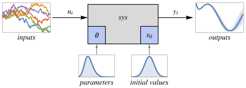
plots the uncertainty in outputs in the system model sys from uncertainty in inputs according to spec.
Details and Options
- SystemModelUncertaintyPlot is typically used to visualize the uncertainty of key signals in a system model resulting from uncertainty in parameters, initial values or inputs. This allows for graphical validation of the impact of uncertainties.
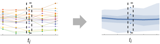
- Given the uncertain parameters, initial values and inputs, the system is simulated a large number of times and a slice function is applied at every point in time to compute aggregate statistics. By default, quantiles are used as a slice function.
- The system model sys can have the following forms:
-
SystemModel[…] general system model StateSpaceModel[…] state-space model TransferFunctionModel[…] transfer function model AffineStateSpaceModel[…] affine state-space model NonlinearStateSpaceModel[…] nonlinear state-space model DiscreteInputOutputModel[…] discrete input-output model - spec is an Association that allows the following keys:
-
"InitialValues" {v1val1,…} variable vi has initial value vali "Inputs" {in1fun1,…} input ini has value funi "Outputs" {v1,…} variables to plot "ParameterValues" {p1val1,…} parameter pi has value vali "SimulationCount" 200 target number of simulations "SimulationInterval" {tmin,tmax} simulate and plot from time tmin to tmax "SliceFunction" sfun function to compute for each time slice - When multiple sources of uncertainty are provided, simulations are performed covering their combinations, using the target number of simulations as an upper bound.
- The values vali in "ParameterValues" and "InitialValues" can take the following forms:
-
pval a single value {pval1,…} custom list of values randomly sampled int an Interval or CenteredInterval uniformly sampled dist an Around or a distribution to sample reg a region to sample uniformly - Multidimensional regions and distributions vald for sets of d variables can be set with {v1,…,vd}vald.
- The inputs funi in "Inputs" can take the following forms:
-
f a single function f[t] at time t {f1,…} a custom list of functions randomly sampled rproc a random process to sample - Vector-valued functions and processes fund for sets of d inputs can be set with {in1,…,ind}fund.
- The slice function sfun can take the following forms:
-
"MinMax" min and max "Quantiles" quantiles 0%, 25%, 50%, 75%, 100% {"Quantiles",{q1,…}} quantiles {q1,…} "Confidence" mean and 95% confidence bands {"Confidence",{cl1,…}} confidence bands with confidence levels {cl1,…} {sfun1,…} list of custom scalar-valued functions - SystemModelUncertaintyPlot has the same options as ListLinePlot, with the following additions and changes: [List of all options]
-
AxesLabel Automatic indicate units on the axis Filling Automatic filling to insert under each curve FrameLabel Automatic frame labels Method Automatic what simulation and plot methods to use PlotLabel Automatic overall label for the plot PlotLayout Automatic how to position data PlotLegends Automatic legends for curves ProgressReporting $ProgressReporting control display of progress SamplingPeriod Automatic sample period for random processes TargetUnits Automatic units to display in the plot - Method settings take the form Method <"sub1"val1,…>.
- Method suboptions "subi" include:
-
"PlotMethod" Automatic plot method "SimulationMethod" Automatic simulation method - "PlotMethod" settings are the same as the Method settings in ListLinePlot.
- "SimulationMethod" settings are the same as the Method settings in SystemModelSimulate.
- SystemModelUncertaintyPlot uses the output as a plot label in the default PlotLayout.
- With PlotLayout "Association", SystemModelUncertaintyPlot gives an Association with the output as the key and its corresponding plot as the value for each requested variable.
- Possible settings for TargetUnits include:
-
None no unit "Unit" unit defined in model "DisplayUnit" display unit defined in model (default) unit explicit unit {unitt,unit} units for time and data - Models with "Epoch" in their simulation settings trigger the use of DateScale.
List of all options
Examples
open all close allBasic Examples (1)
Scope (24)
Models (4)
Plot uncertainty in two variables of a SystemModel:
SystemModelUncertaintyPlot[[image], <|"Outputs" -> {"x", "y"}, "ParameterValues" -> {"theta" -> Interval[{0, π}]}|>, PlotRange -> All]Plot the uncertainty in the output of an AffineStateSpaceModel:
SystemModelUncertaintyPlot[AffineStateSpaceModel[{{Cos[x2], -1/10*x2 - Cos[x1^2]},
  {{0}, {1}}, {x2}, {{0}}}, {x1, x2}, Automatic,
 {Automatic}, Automatic, SamplingPeriod -> None], <|"InitialValues" -> {x1 -> Interval[{1, 2}]}, "SimulationInterval" -> 3|>]
Plot the uncertainty in the output of a NonlinearStateSpaceModel:
SystemModelUncertaintyPlot[NonlinearStateSpaceModel[{{Cos[x] + 4*a*Sin[x/2]},
  {x + Sin[x]}}, {x}, {}, {Automatic}, Automatic,
 SamplingPeriod -> None], <|"ParameterValues" -> {a -> Interval[{1, 10}]}|>]
Plot the uncertainty in the output of a DiscreteInputOutputModel:
diom = DiscreteInputOutputModel[Association["SampledSeries" -> TemporalData[TimeSeries,
    {{{{u[0] + y[-2] + a*y[-1]}, {u[-1] + u[0] + u[1]}}}, {{0, 1, 1}}, 1, {"Discrete", 1},
     {"Discrete", 1}, {1}, {MissingDataMethod -> None, ResamplingMethod -> ... ime", "LastValue", "OutputCount", "OutputVariables", "Path",
  "PathComponent", "PathComponents", "PathFunction", "PathLength", "SamplingPeriod", "StateCount",
  "TemporalData", "TimePath", "Times", "TimeSeries", "TimeValues", "Type", "Values"}];
Use a SquareWave input:
SystemModelUncertaintyPlot[diom, <|"ParameterValues" -> {a -> Interval[{0.1, 1}]}, "Inputs" -> {1 -> SquareWave}|>, PlotRange -> All]Specification (4)
Plot the uncertainty for a specific output:
SystemModelUncertaintyPlot[[image], <|"Outputs" -> {"x"}, "ParameterValues" -> {"theta" -> Interval[{0, π}]}|>, PlotRange -> All]Plot the uncertainty in a model using a custom number of simulations:
SystemModelUncertaintyPlot[[image], <|"SimulationCount" -> 5, "Outputs" -> {"x", "y"}, "ParameterValues" -> {"theta" -> Interval[{0, π}]}|>, PlotRange -> All]Plot the uncertainty for a specific output using a custom simulation interval:
SystemModelUncertaintyPlot[[image], <|"Outputs" -> {"x"}, "SimulationInterval" -> {0, 3}, "ParameterValues" -> {"theta" -> Interval[{0, π}]}|>, PlotRange -> All]Models with "Epoch" in their simulation settings are plotted as values at a sequence of dates:
model = SystemModel[[image], <|"ModelName" -> "MyModel", "SimulationSettings" -> {"Epoch" -> Now, "StopTime" -> Quantity[3, "Hours"]}|>]SystemModelUncertaintyPlot[model, <|"Outputs" -> {"room.temperature.T"}, "ParameterValues" -> {"room.roomInertia.C" -> Range[70000, 90000, 5000]}|>]Uncertainty in Values (5)
Plot the uncertainty generated from giving a list of values for a parameter:
SystemModelUncertaintyPlot[[image], <|"Outputs" -> {"x"}, "ParameterValues" -> {"theta" -> Range[0, 1 / 2, 1 / 200]}|>, PlotRange -> All]Plot the uncertainty generated from sampling an interval for a parameter value:
SystemModelUncertaintyPlot[[image], <|"Outputs" -> {"x"}, "ParameterValues" -> {"theta" -> Interval[{0, 2π}]}|>, PlotRange -> All]Plot the uncertainty generated from sampling a distribution for a parameter value:
SystemModelUncertaintyPlot[[image], <|"Outputs" -> {"x"}, "ParameterValues" -> {"theta" -> NormalDistribution[2, 0.1]}|>, PlotRange -> All]Plot the uncertainty generated from sampling a geometric region for a parameter value:
SystemModelUncertaintyPlot[[image], <|"Outputs" -> {"x"}, "ParameterValues" -> {"theta" -> MeshRegion[{{0}, {1}, {2}}, Line[{1, 2, 3}]]}|>, PlotRange -> All]Plot the uncertainty generated from sampling a Circle for two initial values:
SystemModelUncertaintyPlot[[image], <|"Outputs" -> {"x", "y"}, "InitialValues" -> {{"x", "y"} -> Circle[]}|>, PlotRange -> All]Uncertainty in Inputs (3)
Plot the uncertainty generated when an ARIMAProcess is used for an input:
SystemModelUncertaintyPlot[[image], <|"SimulationInterval" -> {0, 10}, "Outputs" -> {"syse.sys.rs"}, "Inputs" -> {"T" -> ARIMAProcess[{-.01}, 1, {.01}, 10^-6]}|>, PlotRange -> All, TargetUnits -> "Millimeters"]Plot the uncertainty generated when several functions are used as input:
inputs = Table[With[{k = k}, Function[t, 0.1(k Tanh[t] + 0.1k Sin[0.15t])]], {k, 1, 10}];Plot[Through[inputs[x]], {x, 0, 60}]Use these profiles for the input flow rate in a continuous stirred tank reactor:
SystemModelUncertaintyPlot[[image], <|"Inputs" -> {"deltaFJ" -> inputs}|>, PlotRange -> All]Plot the uncertainty generated when using a two-dimensional process for two inputs:
SystemModelUncertaintyPlot[\!\(\*GraphicsBox[«8»]\), <|"Outputs" -> {"w"}, "Inputs" -> {{"V", "TL"} -> MAProcess[{{{.2, .1}, {-.1, .2}}}, {{0.001, 0}, {0, 0.001}}]}|>, PlotRange -> All]Slice Function (4)
Plot the range between the minimum and maximum of the temporal data:
SystemModelUncertaintyPlot[[image], <|"Outputs" -> {"x"}, "ParameterValues" -> {"theta" -> Interval[{0, 2π}]}, "SliceFunction" -> "MinMax"|>, PlotRange -> All]Plot custom quantiles of the temporal data:
SystemModelUncertaintyPlot[[image], <|"Outputs" -> {"x"}, "ParameterValues" -> {"theta" -> Interval[{0, 2π}]}, "SliceFunction" -> {"Quantiles", {0, 0.45, 0.5, 0.55, 1}}|>, PlotRange -> All]Plot confidence bands for the temporal data with custom confidence levels:
SystemModelUncertaintyPlot[[image], <|"Outputs" -> {"x"}, "ParameterValues" -> {"theta" -> Interval[{0, 2π}]}, "SliceFunction" -> {"Confidence", {0.95, 0.98, 0.99}}|>, PlotRange -> All]SystemModelUncertaintyPlot[[image], <|"Outputs" -> {"x"}, "ParameterValues" -> {"theta" -> Interval[{0, 2π}]}, "SliceFunction" -> {Mean[#] - StandardDeviation[#]&, Mean, Mean[#] + StandardDeviation[#]&}|>, PlotRange -> All, PlotLegends -> {μ - σ, μ, μ + σ}]Data Wrappers (4)
Use wrappers on a single variable:
SystemModelUncertaintyPlot[[image], <|"Outputs" -> Style["x", StandardRed], "ParameterValues" -> {"theta" -> Interval[{0, 2π}]}|>]Use wrappers for several variables in a "Shared" PlotLayout:
SystemModelUncertaintyPlot[[image], <|"Outputs" -> {Style["vx", StandardRed], Style["y", StandardOrange]}, "ParameterValues" -> {"theta" -> Interval[{0, 2π}]}|>, PlotLayout -> "Shared"]SystemModelUncertaintyPlot[[image], <|"Outputs" -> Labeled[Style["x", StandardRed], "position", Below], "ParameterValues" -> {"theta" -> Interval[{0, 2π}]}|>]Use wrappers for several variables in a "Shared" PlotLayout:
SystemModelUncertaintyPlot[[image], <|"Outputs" -> {Callout[Style["vx", StandardRed], "velocity", Above], Callout[Style["y", StandardOrange], "position", Below]}, "ParameterValues" -> {"theta" -> Interval[{0, 2π}]}|>, PlotLayout -> "Shared"]Add a Tooltip:
SystemModelUncertaintyPlot[[image], <|"Outputs" -> Tooltip["x", "position"], "ParameterValues" -> {"theta" -> Interval[{0, 2π}]}|>]Customize the plot legend for a single variable:
SystemModelUncertaintyPlot[[image], <|"Outputs" -> Legended["x", "position"], "ParameterValues" -> {"theta" -> Interval[{0, 2π}]}|>]Customize the plot legend for several variables in a "Shared" PlotLayout:
SystemModelUncertaintyPlot[[image], <|"Outputs" -> {Legended["vx", "velocity"], Legended["y", "position"]}, "ParameterValues" -> {"theta" -> Interval[{0, 2π}]}|>, PlotLayout -> "Shared"]Options (17)
AxesLabel (2)
AxesLabel is set to None by default in the default PlotLayout:
SystemModelUncertaintyPlot[[image], <|"Outputs" -> {"x"}, "ParameterValues" -> {"theta" -> Interval[{0, 2π}]}|>, PlotRange -> All, Frame -> False, Axes -> True]SystemModelUncertaintyPlot[[image], <|"Outputs" -> {"x"}, "ParameterValues" -> {"theta" -> Interval[{0, 2π}]}|>, PlotRange -> All, AxesLabel -> {"time", "position"}, Frame -> False, Axes -> True]Filling (2)
Known slice functions use a customized Filling by default:
SystemModelUncertaintyPlot[[image], <|"Outputs" -> {"x"}, "ParameterValues" -> {"theta" -> Interval[{0, 2π}]}|>, PlotRange -> All]SystemModelUncertaintyPlot[[image], <|"Outputs" -> {"x"}, "ParameterValues" -> {"theta" -> Interval[{0, 2π}]}|>, PlotRange -> All, Filling -> {1 -> {5}}]FrameLabel (2)
The units of the plotted variables are used as the FrameLabel by default:
SystemModelUncertaintyPlot[[image], <|"Outputs" -> {"x"}, "ParameterValues" -> {"theta" -> Interval[{0, 2π}]}|>, PlotRange -> All]SystemModelUncertaintyPlot[[image], <|"Outputs" -> {"x"}, "ParameterValues" -> {"theta" -> Interval[{0, 2π}]}|>, FrameLabel -> {"time", "position"}, PlotRange -> All]Method (1)
Set a custom simulation method with Method:
SystemModelUncertaintyPlot[[image], <|"Outputs" -> {"x"}, "ParameterValues" -> {"theta" -> Interval[{0, 2π}]}|>, Method -> <|"SimulationMethod" -> {"InterpolationPoints" -> 10}|>, PlotRange -> All]PlotLabel (1)
PlotLayout (2)
Obtain an Association with individual plots for each output:
SystemModelUncertaintyPlot[[image], <|"Outputs" -> {"x", "vy"}, "ParameterValues" -> {"theta" -> Interval[{0, 2π}]}|>, PlotRange -> All, PlotLayout -> "Association"]SystemModelUncertaintyPlot[[image], <|"Outputs" -> {"x", "vy"}, "ParameterValues" -> {"theta" -> Interval[{0, 2π}]}|>, PlotRange -> All, PlotLayout -> "Shared"]PlotLegends (2)
Known slice functions use customized PlotLegends by default:
SystemModelUncertaintyPlot[[image], <|"Outputs" -> {"x"}, "ParameterValues" -> {"theta" -> Interval[{0, 2π}]}, "SliceFunction" -> {"Quantiles", {0, 0.45, 0.5, 0.55, 1}}|>, PlotRange -> All]SystemModelUncertaintyPlot[[image], <|"Outputs" -> {"x"}, "ParameterValues" -> {"theta" -> Interval[{0, 2π}]}, "SliceFunction" -> {"Quantiles", {0, 0.45, 0.5, 0.55, 1}}|>, PlotLegends -> {None, None, "Median", None, None}]ProgressReporting (1)
Control progress reporting with ProgressReporting:
SystemModelUncertaintyPlot[[image], <|"Outputs" -> {"x"}, "ParameterValues" -> {"theta" -> Interval[{0, 2π}]}|>, PlotRange -> All, ProgressReporting -> False]SamplingPeriod (1)
Set a custom sampling period when sampling a random process:
SystemModelUncertaintyPlot[[image], <|"SimulationInterval" -> {0, 10}, "Outputs" -> {"syse.sys.rs"}, "Inputs" -> {"T" -> ARIMAProcess[{-.01}, 1, {.01}, 10^-6]}|>, PlotRange -> All, TargetUnits -> "mm", SamplingPeriod -> 5]ScalingFunctions (2)
Plot the model with log-scaled values using ScalingFunctions:
SystemModelUncertaintyPlot[AffineStateSpaceModel[{{x1, 2*x1}, {{}}},
 {{x1, 1}, {x2, 1}}], <|"Outputs" -> {x1, x2}, "InitialValues" -> {x1 -> {1, 10, 100, 1000}}|>, ScalingFunctions -> "Log"]
Models with "Epoch" in its simulation settings are plotted as values at a sequence of dates:
model = SystemModel[[image], <|"ModelName" -> "MyModel", "SimulationSettings" -> {"Epoch" -> Now}|>]SystemModelUncertaintyPlot[model, <|"Outputs" -> {"H"}, "ParameterValues" -> {"k" -> Range[100, 130, 5]}|>]Use ScalingFunctions{None,Automatic} to produce simulation time plots instead:
SystemModelUncertaintyPlot[model, <|"Outputs" -> {"H"}, "ParameterValues" -> {"k" -> Range[100, 130, 5]}|>, ScalingFunctions -> {None, Automatic}, TargetUnits -> {"Years", Automatic}]Use DateTicksFormat to format for date tick labels:
SystemModelUncertaintyPlot[model, <|"Outputs" -> {"H"}, "ParameterValues" -> {"k" -> Range[100, 130, 5]}|>, ScalingFunctions -> {DateScale[DateTicksFormat -> "YearShort"], Automatic}]TargetUnits (1)
Set custom units with TargetUnits:
SystemModelUncertaintyPlot[[image], <|"Outputs" -> {"x"}, "ParameterValues" -> {"theta" -> Interval[{0, 2π}]}|>, PlotRange -> All, TargetUnits -> {"Seconds", "Decimeters"}]Applications (6)
Trajectories Near Equilibrium (1)
Plot the uncertainty in the angle and angular velocity of a simple damped pendulum when the initial conditions take values near equilibrium points:
model = CreateSystemModel["DampedPendulum", {ω'[t] == -g Sin[θ[t]] / l - b ω[t], θ'[t] == ω[t]}, t, {θ∈"Units.SI.Angle"}, <|"ParameterValues" -> {g -> 10, l -> 1 / 2, b -> 2}|>]When the system starts at rest at small angles, it evolves toward the stable ground position:
SystemModelUncertaintyPlot[model, <|"SimulationInterval" -> 5, "Outputs" -> θ, "InitialValues" -> {θ -> CenteredInterval[0, π / 4]}|>, ...]When the system starts near the unstable fully inverted position, it also evolves toward the ground position:
SystemModelUncertaintyPlot[model, <|"SimulationInterval" -> 5, "Outputs" -> θ, "InitialValues" -> {θ -> Interval[{3π / 4, π - π / 100}]}|>, ...]Plot a few randomly chosen trajectories:
SystemModelUncertaintyPlot[model, <|"SimulationInterval" -> 5, "Outputs" -> θ, "InitialValues" -> {θ -> Interval[{3π / 4, π - π / 100}]}, "SliceFunction" -> Table[With[{k = k}, Part[#, k]&], {k, RandomSample[Range[200], 20]}]|>, ...]System Tolerance (1)
The performance of a circuit depends heavily on its components and parameter tolerances. When the resistance of one of the components in this model of a speaker follows a truncated normal distribution, the variation in the current going through the speaker can be measurable:
SystemModelUncertaintyPlot[[image], <|"Outputs" -> "speaker.l.i", "SimulationInterval" -> Quantity[40, "Milliseconds"], "ParameterValues" -> {"r1.R" -> TruncatedDistribution[{0, ∞}, NormalDistribution[6, 5]]}|>]External disturbances can also affect the performance of a circuit. For instance, the input voltage of the speaker can be affected by high-frequency signals:
inputs = Table[With[{k = k}, Function[{t}, 2.5Sin[2 π t 50] + k Sin[2 π t 2000]]], {k, 0, 0.6, 0.05}];Plot[Through[inputs[t]], {t, 0, 0.01}]Plot the uncertainty in the current of the speaker when affected by these high-frequency disturbances:
SystemModelUncertaintyPlot[[image], <|"Outputs" -> "speaker.l.i", "SimulationInterval" -> Quantity[10, "Milliseconds"], "Inputs" -> {"vi" -> inputs}|>, TargetUnits -> {"Milliseconds", "Milliamperes"}]Validation of Controlled Systems (1)
Validate a controlled ball and beam system by placing the ball away from the stable position:
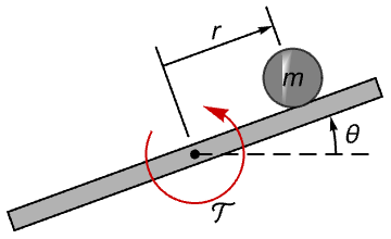
model = [image];The farther away the ball starts from the equilibrium point, the more the system will struggle bringing it back to the stable position:
spec = <|"SimulationInterval" -> {0, 1.2}, "InitialValues" -> {"syse.sys.ballAndBeamDynamics.rs" -> Interval[{0, 0.15}]}|>;SystemModelUncertaintyPlot[model, Append[spec, "Outputs" -> {"syse.sys.ballAndBeamDynamics.rs"}], PlotRange -> All, PlotLabel -> "r"]The control effort peaks at the start and then later a few more times to stop the ball from overshooting the stable position:
SystemModelUncertaintyPlot[model, Append[spec, "Outputs" -> {"syse.sys.T"}], PlotRange -> All, PlotLabel -> "Control effort"]Controlled systems should also be validated against external disturbances. Stress the controlled ball and beam system with a white noise torque disturbance and plot the control effort as the system experiences various sampling periods of the noise:
SystemModelUncertaintyPlot[model, <|"SimulationInterval" -> {0, 1.2}, "Outputs" -> {"syse.sys.T"}, "Inputs" -> {"T" -> WhiteNoiseProcess[0.1]}|>, SamplingPeriod -> 0.3, PlotRange -> All, PlotLabel -> "Control effort"]Orbital Maneuver (1)
Study the effect of a short-time tangential boost on a toy spacecraft in a circular orbit:
model = ConnectSystemModelComponents["BoostModel", {"orbit"∈"Control.CircularOrbit", "zero"∈"Blocks.Sources.Constant", "boost"∈"Blocks.Sources.Pulse"}, {"orbit.fr""zero.y", "orbit.fphi""boost.y"}, IconizedObject[«model settings»]]Boosts of large magnitude can lead to unbounded trajectories:
sim = SystemModelSimulate[model, {"orbit.x", "orbit.y"}, Quantity[8, "Hours"], <|"ParameterValues" -> {"boost.amplitude" -> {0, 600, 700, 800, 900, 1000}}|>];SystemModelPlot[sim, PlotLegends -> None, Axes -> False, Frame -> True]Bounded or unbounded trajectories can unfold if the magnitude of the boost follows a normal distribution. Plot the uncertainty in the distance to the center of force:
SystemModelUncertaintyPlot[model, <|"Outputs" -> {"orbit.r"}, "ParameterValues" -> {"boost.amplitude" -> NormalDistribution[600, 100]}|>]Overshoot in Heating System (1)
Start with a model of a heating system where heat flow switches directions in the middle of the simulation:
model = \!\(\*GraphicsBox[«8»]\);Select the temperature in a pipe as output and specify the simulation interval:
pipe9T = <|"Outputs" -> "pipe9.mediums[1].T", "SimulationInterval" -> 100|>;Choose the diameter of a pipe as parameter and an interval as sampling region:
uncertainty = <|"ParameterValues" -> {"pipe8.diameter" -> Interval[{0.012, 0.055}]}|>;Plot uncertainty in the temperature of a pipe with respect to the diameter of a pipe and see the effect in the overshoot:
SystemModelUncertaintyPlot[model, Join[pipe9T, uncertainty], PlotRange -> {Automatic, {18, 50}}, PlotLabel -> "Temperature overshoot"]Select the temperature in two pipes as outputs:
pipes89T = <|"Outputs" -> {"pipe9.mediums[1].T", "pipe8.mediums[1].T"}, "SimulationInterval" -> 100|>;Plot uncertainty in the temperatures:
SystemModelUncertaintyPlot[model, Join[pipes89T, uncertainty], PlotRange -> All, PlotLayout -> "Shared", PlotLabel -> "Temperature overshoots"]Control Design in Robotics (1)
Start with a model of a robot performing a time-constrained motion carrying a load of 300 kg with a target rotation angle of 60°:
model = SystemModel[\!\(\*GraphicsBox[«8»]\), <|"ParameterValues" -> {"mLoad" -> 300}, "ModelName" -> "IndustrialRobot"|>];Select the rotation angle as output and specify the simulation interval:
angle = <|"Outputs" -> "mechanics.r1.angle", "SimulationInterval" -> 1.856, "InterpolationPoints" -> 500|>;Choose the gain in a controller as the parameter and an interval as sampling region:
uncertainty = <|"ParameterValues" -> {"kp1" -> Interval[{1, 30}]}|>;Plot uncertainty in the rotation angle with respect to the controller gain and see the effect in the target angle at the end of the simulation:
SystemModelUncertaintyPlot[model, Join[angle, uncertainty], PlotRange -> {{1.2, 1.85}, {50, 65}}, PlotLabel -> "Rotation angle", GridLines -> {{}, {60}}]Properties & Relations (2)
Use SystemModelPlot to plot individual curves:
model = \!\(\*GraphicsBox[«8»]\);SystemModelPlot[model, {"Inertia2.w"}, <|"ParameterValues" -> {"Inertia2.J" -> 2}|>]Use SystemModelPlot to plot individual curves when doing a parameter sweep:
SystemModelPlot[model, {"Inertia2.w"}, <|"ParameterValues" -> {"Inertia2.J" -> {1, 2, 3}}|>]Use SystemModelPlot to plot sensitivity bands computed with SystemModelSimulateSensitivity:
sim = SystemModelSimulateSensitivity[model, 10, {"Inertia2.J"}, <|"ParameterValues" -> {"Inertia2.J" -> 2}|>]SystemModelPlot[sim, {{"Inertia2.w", "Inertia2.J", 0.5}}]Use SystemModelUncertaintyPlot to plot uncertainty:
SystemModelUncertaintyPlot[model, <|"Outputs" -> "Inertia2.w", "ParameterValues" -> {"Inertia2.J" -> CenteredInterval[{{1, 1, 536870912, -29}, 63}]}|>]Interval and CenteredInterval are sampled as regions:
model = \!\(\*GraphicsBox[«8»]\);SystemModelUncertaintyPlot[model, <|"Outputs" -> "Inertia2.w", "ParameterValues" -> {"Inertia2.J" -> CenteredInterval[{{1, 1, 858993460, -33}, 66}]}|>]Around and VectorAround are sampled as their corresponding distributions:
SystemModelUncertaintyPlot[model, <|"Outputs" -> "Inertia2.w", "ParameterValues" -> {"Inertia2.J" -> Around[2., 0.1]}|>]Related Links
Text
Wolfram Research (2024), SystemModelUncertaintyPlot, Wolfram Language function, https://reference.wolfram.com/language/ref/SystemModelUncertaintyPlot.html.
CMS
Wolfram Language. 2024. "SystemModelUncertaintyPlot." Wolfram Language & System Documentation Center. Wolfram Research. https://reference.wolfram.com/language/ref/SystemModelUncertaintyPlot.html.
APA
Wolfram Language. (2024). SystemModelUncertaintyPlot. Wolfram Language & System Documentation Center. Retrieved from https://reference.wolfram.com/language/ref/SystemModelUncertaintyPlot.html