


Volume
Volume[reg]
gives the volume of the three-dimensional region reg.
Volume[{x1,…,xn},{s,smin,smax},{t,tmin,tmax},{u,umin,umax}]
gives the volume of the parametrized region whose Cartesian coordinates xi are functions of s, t, u.
Volume[{x1,…,xn},{s,smin,smax},{t,tmin,tmax},{u,umin,umax},chart]
interprets the xi as coordinates in the specified coordinate chart.
Details and Options
- A three-dimensional region can be embedded in any dimension greater than or equal to three.
- In Volume[x,{s,smin,smax},{t,tmin,tmax},{u,umin,umax}], if x is a scalar, Volume returns the volume of the parametric three-region {s,t,u,x}.
- Coordinate charts in the fifth argument of Volume can be specified as triples {coordsys,metric,dim} in the same way as in the first argument of CoordinateChartData. The short form in which dim is omitted may be used.
- The following options can be given:
-
AccuracyGoal Infinity digits of absolute accuracy sought Assumptions $Assumptions assumptions to make about parameters GenerateConditions Automatic whether to generate conditions on parameters PerformanceGoal $PerformanceGoal aspects of performance to try to optimize PrecisionGoal Automatic digits of precision sought WorkingPrecision Automatic the precision used in internal computations - Symbolic limits of integration are assumed to be real and ordered. Symbolic coordinate chart parameters are assumed to be in range given by the "ParameterRangeAssumptions" property of CoordinateChartData.
Examples
open all close allBasic Examples (4)
The volume of a unit ball in 3D:
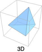
Volume[Ball[]]Region[Ball[]]The volume of a standard simplex in 3D:
Volume[Simplex[3]]Region[Simplex[3]]The volume of a rectangular cuboid:
Volume[{s, t, u}, {s, 0, a}, {t, 0, b}, {u, 0, c}]Volume of the cylinder ![]() ,
, ![]() expressed in cylindrical coordinates:
expressed in cylindrical coordinates:
Volume[{r, t, z}, {r, 0, R}, {t, 0, 2Pi}, {z, 0, zMax}, "Cylindrical"]Scope (23)
Special Regions (7)
Volume of a Cuboid:
Volume[Cuboid[{Subscript[l, x], Subscript[l, y], Subscript[l, z]}, {Subscript[u, x], Subscript[u, y], Subscript[u, z]}]]ℛ = Cuboid[{0, 0, 0}, {3, 2, 1}];
Volume[ℛ]Region[ℛ]ℛ = Parallelepiped[{0, 0, 0}, {{1, 0, 0}, {1, 1, 0}, {0, 1, 1}}];
Volume[ℛ]Region[ℛ]Simplex in 3D:
Volume[Simplex[3]]Region[Simplex[3]]A volume simplex embedded in 4D:
Volume[Simplex[{{0, 0, 0, 0}, {0, 0, 1, 1}, {1, 1, 0, 0}, {0, 1, 1, 0}}]]Ball:
Volume[Ball[{Subscript[c, x], Subscript[c, y], Subscript[c, z]}, r]]ℛ = Ball[{0, 0, 0}, 1];
Volume[ℛ]Region[ℛ]Volume[Ellipsoid[{Subscript[c, x], Subscript[c, y], Subscript[c, z]}, {Subscript[r, x], Subscript[r, y], Subscript[r, z]}]]ℛ = Ellipsoid[{0, 0, 0}, {3, 2, 1}];
Volume[ℛ]Region[ℛ]Volume[Cylinder[{{Subscript[x, 1], Subscript[y, 1], Subscript[z, 1]}, {Subscript[x, 2], Subscript[y, 2], Subscript[z, 2]}}, r]]ℛ = Cylinder[{{0, 0, 0}, {0, 0, 2}}, 1];
Volume[ℛ]Region[ℛ]Cone:
Volume[Cone[{{Subscript[x, 1], Subscript[y, 1], Subscript[z, 1]}, {Subscript[x, 2], Subscript[y, 2], Subscript[z, 2]}}, r]]ℛ = Cone[{{0, 0, 0}, {0, 0, 2}}, 1];
Volume[ℛ]Region[ℛ]Formula Regions (2)
The volume of a ball represented as an ImplicitRegion:
Volume[ImplicitRegion[x^2 + y^2 + z^2 ≤ 1, {x, y, z}]]Volume[ImplicitRegion[x^2 + y^2 ≤ 1, {x, y, {z, 0, 2}}]]The volume of a ball represented as a ParametricRegion:
ℛ = ParametricRegion[{r Cos[θ]Cos[ϕ], r Sin[θ]Cos[ϕ], r Sin[ϕ]}, {{θ, 0, 2π}, {ϕ, -π / 2, π / 2}, {r, 0, 1}}];Volume[ℛ]A cylinder represented with a rational parametrization:
Volume[ParametricRegion[{r(1 - t^2/1 + t^2), r(2t/1 + t^2), z}, {t, {r, 0, 1}, {z, 0, 2}}]]Mesh Regions (2)
The volume of a MeshRegion:
DelaunayMesh[RandomReal[1, {20, 3}]]Volume[%]The volume of a BoundaryMeshRegion:
ConvexHullMesh[RandomReal[1, {20, 3}]]Volume[%]Derived Regions (3)
The volume of a RegionIntersection:
ℛ = RegionIntersection[Ball[{0, 0, 0}, 1], Ball[{0, 0, 1}, 1]];Region[ℛ]Volume[ℛ]The volume of a TransformedRegion:
ℛ = TransformedRegion[Ball[{0, 0, 0}, 1], ScalingTransform[{a, b, c}]];Region[ℛ /. Thread[{a, b, c} -> {3, 2, 1}]]Volume[ℛ]The volume of a RegionBoundary:
RegionBoundary[Ball[{0, 0, 0, 0}, 1]]Volume[%]Parametric Formulas (6)
The volume of an ellipsoid with semimajor axes 3, 2, and 1:
Volume[{3r Cos[ψ], 2r Sin[θ]Sin[ψ], r Cos[θ]Sin[ψ]}, {r, 0, 1}, {θ, 0, 2Pi}, {ψ, 0, Pi}]ParametricPlot3D[{3 Cos[ψ], 2Sin[θ]Sin[ψ], Cos[θ]Sin[ψ]}, {θ, 0, 2Pi}, {ψ, 0, Pi}]The volume of a hemispherical shell in spherical coordinates:
Volume[{r, t, p}, {r, 1, 2}, {t, 0, Pi / 2} , {p, 0, 2Pi}, "Spherical"]ParametricPlot3D[CoordinateTransform[ "Spherical" -> "Cartesian", {r, t, p}] /. {{r -> 1}, {r -> 2}}//Evaluate, {t, 0, Pi / 2}, {p, 0, 2Pi}, PlotTheme -> "Minimal", PlotStyle -> Opacity[.5]]The volume of a torus of major radius 5 and minor radius 2:
Volume[{(5 + 2 r Sin[p])Cos[t], (5 + 2 r Sin[p])Sin[t], 5 Cos[p]}, {r, 0, 1}, {t, 0, 2Pi}, {p, 0, 2Pi} ]ParametricPlot3D[{(5 + 2Sin[p])Cos[t], (5 + 2Sin[p])Sin[t], 2Cos[p]}, {t, 0, 2Pi}, {p, 0, 2Pi} ]The volume of the product of a disk and a circle embedded in four-dimensional space:
Volume[{3r Sin[t], 3r Cos[t], 2Sin[p], 2 Cos[p]}, {r, 0, 1}, {t, 0, 2Pi}, {p, 0, 2Pi}]The volume of the paraboloid ![]() over the rectangle
over the rectangle ![]() :
:
Volume[w ^ 2 + x ^ 2 + y ^ 2, {w, -1, 1.}, {x, -2, 2.}, {y, -3, 3.}]Volume of one octant of a three-sphere using stereographic coordinates:
Volume[{s, t, u}, {s, 0, ∞}, {t, 0, ∞}, {u, 0, ∞}, {"Stereographic", {"Sphere", 1}}]CSG Regions (1)
Volume of a linear CSGRegion:
CSGRegion["Difference", {Cube[2], Cube[{1, 0, 1}, 3]}]Volume[%]CSGRegion["Intersection", {Ball[], Ball[{0, 0, 1}]}]SurfaceArea[%]Subdivision Regions (2)
Volume of a SubdivisionRegion:
SubdivisionRegion[Cube[]]Volume[%]The volume of successive subdivision levels converges to that of the limit region:
levels = Table[SubdivisionRegion[Cube[], i], {i, 0, 3}]ListPlot[Volume /@ levels, ...]Options (6)
AccuracyGoal (1)
Consider a region whose volume is difficult to compute exactly:
ℛ = Region@ImplicitRegion[(x^2 + (9/4)y^2 + z^2 - 1)^3 - x^2z^3 - (9/80)y^2z^3 <= 0, {x, y, z}]volume1 = Volume[ℛ]The AccuracyGoal option can be used to change the default absolute tolerance. Here, the volume computation stops once the accuracy goal criterion has been exceeded:
volume2 = Volume[ℛ, AccuracyGoal -> 3]The result with the default settings is different since the default uses only a precision criterion:
volume1 - volume2Assumptions (1)
The area of an elliptic pyramid with arbitrary semimajor axis ![]() , semiminor axis
, semiminor axis ![]() , and height
, and height ![]() :
:
Volume[{(1 - z / c) r a Cos[t], (1 - z / c) r b Sin[t], z}, {r, 0, 1}, {t, 0, 2Pi}, {z, 0, c}]Adding an assumption that the semiaxes are positive simplifies the answer:
Volume[{(1 - z / c) r a Cos[t], (1 - z / c) r b Sin[t], z}, {r, 0, 1}, {t, 0, 2Pi}, {z, 0, c}, Assumptions -> a > 0 && b > 0]Block[{a = 3, b = 2, c = 5}, RegionPlot3D[ParametricRegion[{(1 - z / c )r a Cos[t], (1 - z / c) r b Sin[t], z}, {{r, 0, 1}, {t, 0, 2Pi}, {z, 0, 5}}], Axes -> True, PlotPoints -> 51, PlotRange -> {{-a, a}, {-a, a}, {0, c}}]]PrecisionGoal (1)
The number of effective digits of precision that should be sought can be specified with PrecisionGoal:
Table[Volume[ImplicitRegion[(x^2 + (9/4)y^2 + z^2 - 1)^3 - x^2z^3 - (9/80)y^2z^3 <= 0, {x, y, z}], PrecisionGoal -> prec], {prec, 1, 5}]Plot the volumes computed for various precision settings:
ListPlot[%, PlotRange -> All]PerformanceGoal (1)
Consider a region whose volume is difficult to compute exactly:
ℛ = Region@ImplicitRegion[(x^2 + (9/4)y^2 + z^2 - 1)^3 - x^2z^3 - (9/80)y^2z^3 <= 0, {x, y, z}]Use PerformanceGoal"Speed" to attempt to compute a volume quickly:
(volume1 = Volume[ℛ, PerformanceGoal -> "Speed"])//TimingUse PerformanceGoal"Performance" to attempt to compute a result with as many correct digits as possible:
(volume2 = Volume[ℛ, PerformanceGoal -> "Quality"])//TimingWorkingPrecision (2)
Compute the Volume using machine arithmetic:
Volume[ImplicitRegion[x ^ 4 + y ^ 4 + z ^ 4 - x y z <= 1, {x, y, z}], WorkingPrecision -> MachinePrecision]In some cases, the exact answer cannot be computed:
Volume[ImplicitRegion[x ^ 4 + y ^ 4 + z ^ 4 - x y z <= 1, {x, y, z}], WorkingPrecision -> ∞]Find the Volume using 30 digits of precision:
Volume[{a Cos[t], a Sin[t], b Sin[t]}, {t, 0, 2Pi}, {a, 0, 1}, {b, 0, 1}, WorkingPrecision -> 30]Applications (6)
f[x_, y_, z_] := x y + z;ℛ = ParametricRegion[{x, y, z, f[x, y, z]}, {{x, 0, 1}, {y, 0, 1}, {z, 0, 1}}];RegionDimension[ℛ]Volume[ℛ]Volume[f[x, y, z], {x, 0, 1}, {y, 0, 1}, {z, 0, 1}]Compute the volume of a polyhedron:
ℛ = PolyhedronData["Tetrahedron", "Polyhedron"]Volume[ℛ]The shape of the Earth is nearly that of an oblate spheroid with volume:
Volume[{ξ, η, φ}, {η, 0, Pi}, {φ, 0, 2Pi}, {ξ, 0, ArcTanh[b / a]}, {{"OblateSpheroidal", aSqrt[1 - (b^2/a^2)]}}]Substitute in the values for the semimajor and semiminor axes:
% /. {a -> GeodesyData["ITRF00", "SemimajorAxis"], b -> GeodesyData["ITRF00", "SemiminorAxis"]}Find the mass of methanol in a Ball:
ℛ = Ball[{0, 0, 0}, Quantity[3, "Centimeters"]];ChemicalData["Methanol", "Density"]Volume[ℛ]Find the mean density of a Cone with a non-uniform mass density defined by ![]() :
:
ℛ = Cone[{{0, 0, 0}, {0, 0, h}}, r];Simplify[Integrate[x ^ 2 + y ^ 2 + z ^ 2, Element[{x, y, z}, ℛ]] / Volume[ℛ], h > 0 && r > 0]Compute the volume of empty space in a can with ![]() tennis balls, each with a radius of 1.75 inches:
tennis balls, each with a radius of 1.75 inches:
r = Quantity[1.75, "Inches"];
height = 2 n r;can = Cylinder[{{0, 0, 0}, {0, 0, height}}, r];
ball = Ball[{0, 0, 0}, r];Volume[can] - n Volume[ball]Visualize a can of three balls:
n = 3;Graphics3D[{{Opacity[0.3], can}, Table[Ball[{0, 0, 2 r k - r}, r], {k, n}]} /. q_Quantity :> QuantityMagnitude[q], Boxed -> False]Properties & Relations (5)
Volume is a non-negative quantity:
Volume[{r Cos[φ] Sin[θ], r Sin[θ] Sin[φ], r Cos[θ]}, {r, 0, 1}, {θ, 0, π}, {φ, 0, 2Pi}]Volume[{r Cos[φ] Sin[θ], r Sin[θ] Sin[φ], r Cos[θ]}, {r, 0, 1}, {θ, 0, π}, {φ, 0, -2Pi}]Volume[r] is the same as RegionMeasure[r] for 3D regions:
ℛ = Ball[3];{Volume[ℛ], RegionMeasure[ℛ]}Volume[r] is the same as RegionMeasure[r,3] in general:
{Volume[Sphere[{0, 0, 0, 0}]], RegionMeasure[Sphere[{0, 0, 0, 0}], 3]}Volume[x,s,t,u,c] is equivalent to RegionMeasure[x,{s,t,u},c]:
Volume[{s t ^ 2, Pi / 2, u, s t}, {s, 0, 1}, {t, 0, 2Pi}, {u, 0, 1}, "Hyperspherical"]RegionMeasure[{s t ^ 2, Pi / 2, u, s t}, {{s, 0, 1}, {t, 0, 2Pi}, {u, 0, 1}}, "Hyperspherical"]For a 3D region, Volume is defined as the integral of 1 over that region:
ℛ = Ellipsoid[{1, 2, 3}, {4, 5, 6}];
{Volume[ℛ], Integrate[1, x∈ℛ]}
To get the surface volume of a 4D region, use RegionBoundary:
ℛ = Ball[4];
Volume[RegionBoundary[ℛ]]
Possible Issues (2)
The parametric form of Volume computes the volume of possibly multiple coverings:
Volume[{r Cos[φ] Sin[θ], r Sin[θ] Sin[φ], r Cos[θ]}, {r, 0, 1}, {θ, 0, π}, {φ, 0, 10Pi}]The region version computes the volume of the image:
Volume[ParametricRegion[{r Cos[φ] Sin[θ], r Sin[θ] Sin[φ], r Cos[θ]}, {{r, 0, 1}, {θ, 0, π}, {φ, 0, 10Pi}}]]Volume[Ball[{0, 0, 0}, 1]]The volume of a region of dimension other than 3 is Undefined:
{Volume[Point[{0, 0}]], Volume[Circle[]], Volume[Ball[{0, 0, 0, 0}, 1]]}RegionDimension /@ {Point[{0, 0}], Circle[], Ball[{0, 0, 0, 0}, 1]}Text
Wolfram Research (2014), Volume, Wolfram Language function, https://reference.wolfram.com/language/ref/Volume.html (updated 2019).
CMS
Wolfram Language. 2014. "Volume." Wolfram Language & System Documentation Center. Wolfram Research. Last Modified 2019. https://reference.wolfram.com/language/ref/Volume.html.
APA
Wolfram Language. (2014). Volume. Wolfram Language & System Documentation Center. Retrieved from https://reference.wolfram.com/language/ref/Volume.html