


RegionMeasure
RegionMeasure[reg]
gives the measure of the region reg.
RegionMeasure[reg,d]
gives the d-dimensional measure of the region reg.
RegionMeasure[{x1,…,xn},{{t1,a1,b1},…,{tk,ak,bk}}]
gives the k-measure of the parametric formula whose Cartesian coordinates xi are functions of tj.
RegionMeasure[{x1,…,xn},{{t1,a1,b1},…,{tk,ak,bk}},chart]
interprets the xi as coordinates in the specified coordinate chart.
Details and Options
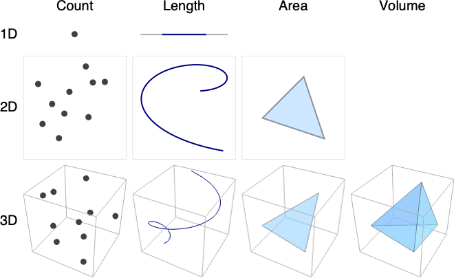
- RegionMeasure is also known as count (0D), length (1D), area (2D), volume (3D), and Lebesgue measure.
- Example cases where rows correspond to embedding dimension and columns to geometric dimension:
- If the region reg is of dimension d≥0, then the d-dimensional measure is used.
- The zero-dimensional measure counts the number of points in the region.
- In RegionMeasure[x,{{t1,a1,b1},…,{tk,ak,bk}}], if x is a scalar, RegionMeasure returns the measure of the hypersurface {t1,…,tk,x} in k+1 dimensions.
- Coordinate charts in the third argument of RegionMeasure can be specified as triples {coordsys,metric,dim} in the same way as in the first argument of CoordinateChartData. The short form in which dim is omitted may be used.
- The following options can be given:
-
AccuracyGoal Infinity digits of absolute accuracy sought Assumptions $Assumptions assumptions to make about parameters GenerateConditions Automatic whether to generate conditions on parameters PerformanceGoal $PerformanceGoal aspects of performance to try to optimize PrecisionGoal Automatic digits of precision sought WorkingPrecision Automatic the precision used in internal computations - Symbolic limits of integration are assumed to be real and ordered. Symbolic coordinate chart parameters are assumed to be in range given by the "ParameterRangeAssumptions" property of CoordinateChartData.
- RegionMeasure can be used with symbolic regions in GeometricScene.
Examples
open all close allBasic Examples (6)
RegionMeasure corresponds to count for zero-dimensional regions:
ℛ = Point[{{0, 0}, {1, 0}, {1, 1}}];RegionDimension[ℛ]RegionMeasure[ℛ]RegionMeasure corresponds to curve length for one-dimensional regions:
ℛ = Line[{{0, 0, 0}, {1, 1, 1}}];RegionDimension[ℛ]RegionMeasure[ℛ]ArcLength[ℛ]RegionMeasure corresponds to surface area for two-dimensional regions:
ℛ = Disk[];RegionDimension[ℛ]RegionMeasure[ℛ]Area[ℛ]RegionMeasure corresponds to volume for three-dimensional regions:
ℛ = Ball[];RegionDimension[ℛ]RegionMeasure[ℛ]Volume[ℛ]RegionMeasure[{r Cos[x], r Sin[2x]}, {{x, 0, 2π}, {r, 1 / 2, 1}}]ParametricPlot[{r Cos[x], r Sin[2x]}, {x, 0, 2π}, {r, 1 / 2, 1}]Volume of a cylinder expressed in cylindrical coordinates:
RegionMeasure[{r, t, z}, {{r, 0, R}, {t, 0, 2Pi}, {z, 0, Z}}, "Cylindrical"]Scope (29)
Special Regions (10)
The measure for Point corresponds to counts:
ℛ = Point[Tuples[Range[5], 2]];
Region[ℛ]RegionMeasure[ℛ]Points can be used in any number of dimensions:
RegionMeasure[Point[Tuples[Range[5], 4]]]The measure for Line corresponds to arc length:
ℛ = Line[{{0, 0}, {1, 1}}];
Region[ℛ]RegionMeasure[ℛ]Lines can be used in any number of dimensions:
RegionMeasure[Line[{{0}, {1}}]]RegionMeasure[Line[{{0, 0, 0}, {1, 1, 1}}]]Rectangle can be used in 2D, and the measure corresponds to area:
RegionMeasure[Rectangle[{Subscript[l, x], Subscript[l, y]}, {Subscript[u, x], Subscript[u, y]}]]Region[Rectangle[{0, 0}, {2, 1}]]Cuboid can be used in any number of dimensions:
RegionMeasure[Cuboid[{Subscript[l, x], Subscript[l, y], Subscript[l, z]}, {Subscript[u, x], Subscript[u, y], Subscript[u, z]}]]Region[Cuboid[{0, 0, 0}, {3, 2, 1}]]RegionMeasure[Cuboid[{Subscript[l, x], Subscript[l, y], Subscript[l, z], Subscript[l, w]}, {Subscript[u, x], Subscript[u, y], Subscript[u, z], Subscript[u, w]}]]A Simplex can correspond to a point, line, or triangle in 2D:
ℛ = {Simplex[{{0, 0}}], Simplex[{{0, 0}, {1, 1}}], Simplex[{{0, 0}, {1, 0}, {0, 1}}]};Table[Region[s], {s, ℛ}]RegionMeasure /@ ℛSimplices can be used in any number of dimensions:
RegionMeasure[Simplex[{{0}, {1}}]]RegionMeasure[Simplex[{{0, 0, 0}, {1, 0, 0}, {0, 1, 0}, {0, 0, 1}}]]The measure of a standard unit simplex in dimension ![]() :
:
Table[RegionMeasure[Simplex[n]], {n, 1, 7}]Polygon represents an area:
ℛ = Polygon[{{0, 0}, {2, -1}, {1, 0}, {2, 1}}];
Region[ℛ]RegionMeasure[ℛ]ℛ = Polygon[{{0, 0, 0}, {(5/3), (2/3), -(4/3)}, {(2/3), (2/3), -(1/3)}, {1, 2, 0}}];
Region[ℛ]RegionMeasure[ℛ]Disk can be used in 2D:
RegionMeasure[Disk[{Subscript[c, x], Subscript[c, y]}, r]]Region[Disk[{0, 0}, 1]]Ball can be used in any dimension, and the measure is the generalized volume:
RegionMeasure[Ball[{Subscript[c, x], Subscript[c, y], Subscript[c, z]}, r]]Region[Ball[{0, 0, 0}, 1]]The measure of unit balls in dimension ![]() :
:
Table[RegionMeasure[Ball[n]], {n, 1, 7}]Disk as an ellipse can be used in 2D:
RegionMeasure[Disk[{Subscript[c, x], Subscript[c, y]}, {Subscript[r, x], Subscript[r, y]}]]Region[Disk[{0, 0}, {3, 2}]]Ellipsoid can be used in any dimension:
RegionMeasure[Ellipsoid[{Subscript[c, x], Subscript[c, y], Subscript[c, z]}, {Subscript[r, x], Subscript[r, y], Subscript[r, z]}]]Region[Ellipsoid[{0, 0, 0}, {3, 2, 1}]]RegionMeasure[Ellipsoid[{Subscript[c, 1], Subscript[c, 2], Subscript[c, 3], Subscript[c, 4], Subscript[c, 5]}, {Subscript[r, 1], Subscript[r, 2], Subscript[r, 3], Subscript[r, 4], Subscript[r, 5]}]]Circle can be used in 2D:
RegionMeasure[Circle[{Subscript[c, x], Subscript[c, y]}, r]]Region[Circle[{0, 0}, 1]]RegionMeasure[Circle[{Subscript[c, x], Subscript[c, y]}, {Subscript[r, x], Subscript[r, y]}]]Region[Circle[{0, 0}, {3, 2}]]Cylinder can be used in 3D:
RegionMeasure[Cylinder[{{Subscript[x, 1], Subscript[y, 1], Subscript[z, 1]}, {Subscript[x, 2], Subscript[y, 2], Subscript[z, 2]}}, r]]Region[Cylinder[{{0, 0, 0}, {0, 0, 2}}, 1]]Cone can be used in 3D:
RegionMeasure[Cone[{{Subscript[x, 1], Subscript[y, 1], Subscript[z, 1]}, {Subscript[x, 2], Subscript[y, 2], Subscript[z, 2]}}, r]]Region[Cone[{{0, 0, 0}, {0, 0, 2}}, 1]]Formula Regions (2)
The measure of a disk represented as an ImplicitRegion:
RegionMeasure[ImplicitRegion[x^2 + y^2 ≤ 1, {x, y}]]RegionMeasure[ImplicitRegion[x^2 + y^2 ≤ 1, {x, y, {z, 0, 2}}]]The measure of a disk represented as a ParametricRegion:
RegionMeasure[ParametricRegion[{r Cos[θ], r Sin[θ]}, {{r, 0, 1}, {θ, 0, 2π}}]]Using a rational parametrization of disk:
RegionMeasure[ParametricRegion[{r(1 - t^2/1 + t^2), r(2t/1 + t^2)}, {t, {r, 0, 1}}]]RegionMeasure[ParametricRegion[{r Cos[θ], r Sin[θ], z}, {{r, 0, 1}, {θ, 0, 2π}, {z, 0, 2}}]]Mesh Regions (2)
The measure of a MeshRegion in 2D:
DelaunayMesh[RandomReal[1, {10, 2}]]RegionMeasure[%]MeshRegion[{{0, 0}, {1, 0}, {2, -1}, {2, 1}}, {Line[{{1, 2, 3, 4, 2}}]}]RegionMeasure[%]DelaunayMesh[RandomReal[1, {20, 3}]]RegionMeasure[%]The measure of a BoundaryMeshRegion:
ConvexHullMesh[RandomReal[1, {10, 2}]]RegionMeasure[%]ConvexHullMesh[RandomReal[1, {30, 3}]]RegionMeasure[%]Derived Regions (3)
The measure of a RegionIntersection:
ℛ = RegionIntersection[Disk[{0, 0}, 1], Disk[{0, 1}, 1]];Region[ℛ]RegionMeasure[ℛ]The measure of a TransformedRegion:
ℛ = TransformedRegion[Disk[{0, 0}, 1], ShearingTransform[θ, {1, 0}, {0, 1}]];DiscretizeRegion[ℛ /. {θ -> 30Degree}, {{-2, 2}, {-1, 1}}]RegionMeasure[ℛ]The measure of a RegionBoundary:
ℛ = RegionBoundary[Simplex[2]];DiscretizeRegion[ℛ, {{-1.1, 1.1}, {-1.1, 1.1}}]RegionMeasure[ℛ]Geographic Regions (2)
The measure of a polygon of geographic entities:
ℛ = Polygon[["france"]];RegionMeasure[ℛ]Polygons with GeoPosition:
ℛ = Polygon[GeoPosition[{{{40.083441, -88.235716}, {40.083607, -88.257488}, {40.082603, -88.257149},
   {40.076136999999996, -88.25740499999999}, {40.076178, -88.270888}, {40.076516, -88.271558},
   {40.083686, -88.271512}, {40.083659999999995, -88.267046},  ... 33323}, {40.098112, -88.228687},
   {40.095216, -88.228627}, {40.095179, -88.238547}, {40.094480999999995, -88.238546},
   {40.094508999999995, -88.23267}, {40.094106, -88.232556}, {40.090666999999996, -88.232477},
{40.090741, -88.235745}}}]];RegionMeasure[ℛ]The measure of a polygon with GeoGridPosition:
ℛ = Polygon[GeoGridPosition[{{{-0.9950503945490105, 1.2366760550756015},
   {-0.9952074890903578, 1.2369207053693891}, {-0.9952196732768064, 1.2369073327446167},
   {-0.9953160063787643, 1.236848436956935}, {-0.9954141759436825, 1.2369993898475449},
   {-0. ... 197645333103}, {-0.9949098578570917, 1.2368130881428654},
   {-0.9948663952535768, 1.2367477711687371}, {-0.9948714472169538, 1.2367426500757825},
{-0.9949211061652593, 1.2367089232486177}, {-0.9949439717990124, 1.236746107097628}}}, "Bonne"]];RegionMeasure[ℛ]Parametric Formulas (8)
RegionMeasure[{Cos[x], Sin[x]}, {{x, 0, 5 / 4}}]ParametricPlot[{Cos[x], Sin[x]}, {x, 0, 5 / 4}, PlotRange -> {0, 1}]An infinite curve in polar coordinates with finite length:
RegionMeasure[{Exp[-t / 10], t}, {{t, 0, ∞}}, "Polar"]ParametricPlot[CoordinateTransform[ "Polar" -> "Cartesian", {Exp[-t / 10], t}]//Evaluate, {t, 0, 50}, PlotRange -> All]The surface area of a torus of major radius 5 and minor radius 2:
RegionMeasure[{(5 + 2Sin[p])Cos[t], (5 + 2Sin[p])Sin[t], 2Cos[p]}, {{t, 0, 2Pi}, {p, 0, 2Pi}}]RegionMeasure[{(5 + 2 r Sin[p])Cos[t], (5 + 2 r Sin[p])Sin[t], 5 Cos[p]}, {{r, 0, 1}, {t, 0, 2Pi}, {p, 0, 2Pi}}]ParametricPlot3D[{(5 + 2Sin[p])Cos[t], (5 + 2Sin[p])Sin[t], 2Cos[p]}, {t, 0, 2Pi}, {p, 0, 2Pi} ]The area of a "flat torus" embedded in four-dimensional space:
RegionMeasure[{5Sin[t], 5Cos[t], 2Sin[p], 2Cos[p]}, {{t, 0, 2Pi}, {p, 0, 2Pi}}]The hypervolume of a 4-sphere embedded in five dimensions:
RegionMeasure[{Cos[θ], Cos[φ] Sin[θ], Cos[ψ] Sin[θ] Sin[φ], Cos[χ] Sin[θ] Sin[φ] Sin[ψ], Sin[θ] Sin[φ] Sin[χ] Sin[ψ]}, {{θ, 0, Pi}, {φ, 0, Pi}, {ψ, 0, Pi}, {χ, 0, 2Pi}}]The hypervolume of the paraboloidal function graph ![]() over the unit hypercube:
over the unit hypercube:
RegionMeasure[w^2 + x^2 + y^2 + z^2, {{w, 0, 1.}, {x, 0, 1.}, {y, 0, 1.}, {z, 0, 1.}}]The length of a curve "bouncing" between the poles on the unit sphere:
RegionMeasure[{TriangleWave[{0, Pi}, p / (2Pi)], p}, {{p, 0, 2Pi}}, {"Standard", {"Sphere", 1}}]RegionMeasure[{TriangleWave[{0, Pi}, p / (2Pi)], p}, {{p, 0, 2Pi}}, {"Standard", {"Sphere", 1}}]Show[{Graphics3D[{Opacity[.5], Sphere[]}], ParametricPlot3D[Evaluate@CoordinateTransform[ "Spherical" -> "Cartesian", {1, TriangleWave[{0, Pi}, p / (2Pi)], p}], {p, 0, 2Pi}]}]The area of the unit square in stereographic coordinates on the sphere:
RegionMeasure[{x, y}, {{x, 0, 1}, {y, 0, 1}}, {"Stereographic", {"Sphere", 1}}]Show[{Graphics3D[{Opacity[.5], Sphere[]}], ParametricPlot3D[Evaluate@CoordinateTransform[ "Spherical" -> "Cartesian", Prepend[CoordinateTransform[{"Stereographic", {"Sphere", 1}} -> {"Standard", {"Sphere", 1}}, {x, y}], 1]], {x, 0, 1}, {y, 0, 1}]}]CSG Regions (1)
The measure of a CSGRegion in 2D:
ℛ = CSGRegion["Difference", {Disk[], Disk[{1 / 2, 1 / 2}]}]RegionMeasure[ℛ]ℛ = CSGRegion["Difference", {Cube[2], Cylinder[{{1, 1, 1}, {1, -1, 1}}]}]RegionMeasure[ℛ]Subdivision Regions (1)
The measure of a SubdivisionRegion in 2D:
ℛ = SubdivisionRegion[Rectangle[]]RegionMeasure[ℛ]ℛ = SubdivisionRegion[Cube[]]RegionMeasure[ℛ]Options (4)
Assumptions (2)
The implicit region can represent both ellipses and hyperbolas:
RegionMeasure[ImplicitRegion[x ^ 2 + a y ^ 2 == 1, {x, y}], GenerateConditions -> True]Adding the assumption ![]() gives the length of an ellipse only:
gives the length of an ellipse only:
RegionMeasure[ImplicitRegion[x ^ 2 + a y ^ 2 == 1, {x, y}], Assumptions -> a > 0]The area of an ellipse with arbitrary semimajor axes ![]() and
and ![]() :
:
RegionMeasure[{r, v}, {{r, 0, ArcSech[Sqrt[1 - (b^2/a^2)]]}, {v, 0, 2Pi}}, {{"Elliptic", Sqrt[a^2 - b^2]}}]Adding an assumption that the semimajor axes are positive simplifies the answer:
RegionMeasure[{r, v}, {{r, 0, ArcSech[Sqrt[1 - (b^2/a^2)]]}, {v, 0, 2Pi}}, {{"Elliptic", Sqrt[a^2 - b^2]}}, Assumptions -> a > 0 && b > 0]WorkingPrecision (2)
Compute the arc length using machine arithmetic:
RegionMeasure[ImplicitRegion[x ^ 6 + y ^ 6 - x y == 1, {x, y}], WorkingPrecision -> MachinePrecision]Find the area using 30 digits of precision:
RegionMeasure[{a Cos[t], a Sin[t], a Sin[t]}, {{t, 0, 2Pi}, {a, 0, 1}}, WorkingPrecision -> 30]Applications (13)
Points (2)
For point sets, the counting measure is used. Each point contributes 1 to the measure:
pts = Point[Tuples[Range[10], 2]];
Region[pts]RegionMeasure[pts]For constant point mass ![]() , multiply the measure by
, multiply the measure by ![]() to get the total mass:
to get the total mass:
m = 0.5;
pts = Point[Tuples[Range[10], 2]];
m RegionMeasure[pts]
For a varying point mass function ![]() , use Integrate:
, use Integrate:
ρ[x_, y_] := (x^2 + y^2) / 100;Integrate[ρ[x, y], {x, y}∈pts]Curves (4)
The length of a function curve ![]() :
:
RegionMeasure[ParametricRegion[{x, x^2}, {{x, 0, 1}}]]The length of an implicit curve:
RegionMeasure[ImplicitRegion[x^2 + y^2 == 1, {x, y}]]RegionMeasure[ImplicitRegion[x^2 + y^2 == 1∧z == x, {x, y, z}]]Find a formula for the length of a Peano curve:
curves = {[image], [image], [image], [image]};RegionMeasure /@ curvesFindSequenceFunction[Rationalize[%], n]Find the total charge along a wire with constant charge density ![]() :
:
δ = 3 / 10;
r = ImplicitRegion[x^2 + y^2 == 1, {x, y}];
δ RegionMeasure[r]
For varying density ![]() , use Integrate:
, use Integrate:
ρ[x_, y_] := Exp[-x^2];Integrate[ρ[x, y], {x, y}∈r]Surfaces (2)
The area of a function surface ![]() :
:
RegionMeasure[ParametricRegion[{x, y, x y}, {{x, 0, 1}, {y, 0, 1}}]]Total mass for a rectangular region:
ℛ = Rectangle[];δ RegionMeasure[ℛ]With varying mass density given by ![]() , use Integrate:
, use Integrate:
Integrate[x y, {x, y}∈ℛ]Solids (3)
Total mass for a Ball with constant density ![]() :
:
δ RegionMeasure[Ball[3]]For a varying density function ![]() , use Integrate:
, use Integrate:
ρ[x_, y_, z_] := x^2 + y^2 + z^2;Integrate[ρ[x, y, z], {x, y, z}∈Ball[3]]Find the mass of ethanol in a Cone:
ℛ = Cone[{{0, 0, 0}, Quantity[{0, 0, 7}, "Centimeters"]}, Quantity[8, "Centimeters"]];d = ChemicalData["Ethanol", "Density"]v = RegionMeasure[ℛ]FormulaData["MassDensity", {"ρ" -> d, "V" -> v}]Find the mass of a Cylinder with a nonuniform mass density defined by ![]() :
:
ℛ = Cylinder[{{0, 0, 0}, {0, 0, h}}, r];d = Integrate[x ^ 2 + y ^ 2 + z ^ 2, {x, y, z}∈ℛ, Assumptions -> h > 0 && r > 0]v = RegionMeasure[ℛ]FormulaData["MassDensity", {"ρ" -> d, "V" -> v}]Solve[% , M]Higher-Dimensional Regions (2)
Derive a formula for the region measure of an ![]() -dimensional unit ball:
-dimensional unit ball:
Table[RegionMeasure[Ball[n]], {n, 10}]FindSequenceFunction[%, n]The volume of the 3D hypersurface ![]() :
:
RegionMeasure[ParametricRegion[{x, y, z, x^2 + y - z}, {{x, 0, 1}, {y, 0, 1}, {z, 0, 1}}]]Properties & Relations (10)
RegionMeasure for a region ℛ is given by the integral ![]() :
:
ℛ = Circle[];{RegionMeasure[ℛ], Integrate[1, {x, y}∈ℛ]}ℛ = Ball[];{RegionMeasure[ℛ], Integrate[1, {x, y, z}∈ℛ]}ArcLength is a special case of RegionMeasure for one-dimensional regions:
{ArcLength[Circle[]], RegionMeasure[Circle[]]}Area is a special case of RegionMeasure for two-dimensional regions:
{Area[Disk[]], RegionMeasure[Disk[]]}Volume is a special case of RegionMeasure for three-dimensional regions:
{Volume[Ball[]], RegionMeasure[Ball[]]}The measure used is determined by RegionDimension, including count for dimension 0:
ℛ = Point[{0, 0, 0}];{RegionDimension[ℛ], RegionMeasure[ℛ]}ℛ = Line[{{0, 0}, {1, 1}}];{RegionDimension[ℛ], RegionMeasure[ℛ]}ℛ = Triangle[{{0, 0}, {1, 0}, {0, 1}}];{RegionDimension[ℛ], RegionMeasure[ℛ]}ℛ = Tetrahedron[{{0, 0, 0}, {1, 0, 0}, {0, 1, 0}, {0, 0, 1}}];{RegionDimension[ℛ], RegionMeasure[ℛ]}For regions containing a mix of dimensions, RegionDimension gives the largest dimension:
ℛ = RegionUnion[Point[{1, 0}], Line[{{0, 0}, {1, 1}}]];Since the dimension is 1, this computes the length:
{RegionDimension[ℛ], RegionMeasure[ℛ]}RegionMeasure[x,{t},c] is equivalent to ArcLength[x,t,c]:
RegionMeasure[{t ^ 2, Pi / 2, Pi / 4, t}, {{t, 0, 2Pi}}, "Hyperspherical"]ArcLength[{t ^ 2, Pi / 2, Pi / 4, t}, {t, 0, 2Pi}, "Hyperspherical"]RegionMeasure[x,{s,t},c] is equivalent to Area[x,s,t,c]:
RegionMeasure[{s t ^ 2, Pi / 2, Pi / 4, s t}, {{s, 0, 1}, {t, 0, 2Pi}}, "Hyperspherical"]Area[{s t ^ 2, Pi / 2, Pi / 4, s t}, {s, 0, 1}, {t, 0, 2Pi}, "Hyperspherical"]RegionMeasure[x,{s,t,u},c] is equivalent to Volume[x,s,t,u,c]:
RegionMeasure[{s t ^ 2, Pi / 2, u, s t}, {{s, 0, 1}, {t, 0, 2Pi}, {u, 0, 1}}, "Hyperspherical"]Volume[{s t ^ 2, Pi / 2, u, s t}, {s, 0, 1}, {t, 0, 2Pi}, {u, 0, 1}, "Hyperspherical"]RegionCentroid is equivalent to Integrate[p,p∈ℛ]/m with m=RegionMeasure[ℛ]:
ℛ = Ball[{1, 2, 3}];
m = RegionMeasure[ℛ];{RegionCentroid[ℛ], Integrate[{x, y, z}, {x, y, z}∈ℛ] / m}Possible Issues (3)
RegionMeasure uses the counting measure for discrete points:
ℛ = RegionIntersection[Disk[{0, 0}, 1], Disk[{0, 2}, 1]];RegionMeasure[ℛ]This specifies that the two-dimensional Lebesgue measure should be used:
RegionMeasure[ℛ, 2]The parametric form takes the parametrization as fundamental and will count multiple coverings:
RegionMeasure[{Sin[t], Cos[t]}, {{t, 0, 4Pi}}]The region version computes the measure of the image:
RegionMeasure[ParametricRegion[{Sin[t], Cos[t]}, {{t, 0, 4Pi}}]]RegionMeasure uses machine arithmetic when the exact answer cannot be computed:
RegionMeasure[ImplicitRegion[x ^ 6 + y ^ 6 - x y == 1, {x, y}]]Neat Examples (1)
Find the measure of the Cantor set:
ℛℛ = Table[CantorMesh[n], {n, 0, 5}];Column[ℛℛ]Compute the measure for the first six iterations:
RegionMeasure /@ ℛℛ//RationalizeFind the length for iteration k:
FindSequenceFunction[%, k]Limit[%, k -> ∞]Text
Wolfram Research (2014), RegionMeasure, Wolfram Language function, https://reference.wolfram.com/language/ref/RegionMeasure.html (updated 2019).
CMS
Wolfram Language. 2014. "RegionMeasure." Wolfram Language & System Documentation Center. Wolfram Research. Last Modified 2019. https://reference.wolfram.com/language/ref/RegionMeasure.html.
APA
Wolfram Language. (2014). RegionMeasure. Wolfram Language & System Documentation Center. Retrieved from https://reference.wolfram.com/language/ref/RegionMeasure.html