


PointValuePlot
PointValuePlot[{pt1val1,pt2val2,…}]
plots the points pti styled according to the values vali.
PointValuePlot[ptsvals]
uses a collection of points pti from pts with corresponding values vali from val.
PointValuePlot[…,enc]
uses the visual encoding enc to represent the values vali in the plot.
PointValuePlot[data,…]
plots the locations and values from data.
Details and Options
- PointValuePlot is also known as a graduated symbol map and thematic map.
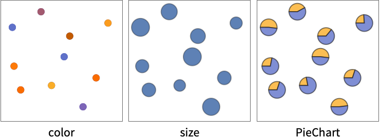
- PointValuePlot uses various visual encodings enc such as color, size and shape to represent values at specific locations.
- The coordinates {x,y} in point pti can be given in the following forms:
-
xi a real-valued number Quantity[xi,unit] a quantity with a unit Around[xi,ei] value xi with uncertainty ei Interval[{xmin,xmax}] values between xmin and xmax - The ptsi can be geographic locations with the following forms:
-
GeoPosition[{lat,lon}] latitude and longitude Entity[…] geographic entity Dated[…] dated entity - Multiple points pts can be given in the following forms:
-
{pt1,pt2,…} list of individual points QuantityArray[…] array of quantities GeoPosition[…] array of geodetic positions - The values vali can be any form, including:
-
n numeric value Quantity[vali,unit] magnitude with units "str" string RGBColor[…],Hue[…],… color {vali1,vali2,…} list of values - Multiple values values can be given in the following forms:
-
{val1,val2,…} list of individual values QuantityArray[{val1,val2,…},unit] array of quantities Dataset[…] dataset of values - The data data for PointValuePlot can be given in the following forms:
-
{e1,e2,…} list of elements with or without wrappers <k1e1,k2e2,…> association of keys and values SpatialPointData[…] spatial points and annotations WeightedData[…] positions with weights for values w[{e1,e2,…},…] wrapper applied to a whole dataset w[{data1,data1,…},…] wrapper applied to all datasets - The following wrappers can be used for plot elements:
-
Annotation[e,label] provide an annotation Button[e,action] define an action to execute when the element is clicked Callout[e,label] label the data with a callout EventHandler[e,…] define a general event handler for the element Hyperlink[e,uri] make the element act as a hyperlink Labeled[e,…] display the element with labeling Legended[e,…] include features of the element in a chart legend PopupWindow[e,cont] attach a popup window to the element StatusArea[e,label] display in the status area when the element is moused over Style[e,opts] show the element using the specified styles Tooltip[e,label] attach an arbitrary tooltip to the element - Data not given in these forms is ignored in forming the plot.
- By default, the encoding enc is automatically chosen based on the forms of the values vali.
- Possible settings for the encoding enc can be:
-
"Size" vary the point sizes according to the values "Color" smoothly color the points according to the values "DiscreteColor" discretely color the points according to the values "Shape" vary the shape of the point according to the values "Label" label the points with the values func apply func to the values to determine the point marker nenc encode the n ") value for a point with the encoding enc
value for a point with the encoding encm;;nenc encode the m ") through n
through n") values with the encoding enc
values with the encoding encAllenc encode all the values for a point with the encoding enc {enc1,enc2,…} use different encodings for different values - PointValuePlot takes the same options as Graphics with the following additions and changes: [List of all options]
-
AspectRatio Automatic overall ratio of width to height Axes Automatic whether to draw axes BubbleScale "Area" feature scale used for bubbles BubbleSizes Automatic size range to use for bubbles ColorFunction Automatic how to determine the color of points ColorFunctionScaling True whether to scale arguments to ColorFunction Frame Automatic whether to draw a frame around the plot GeoBackground Automatic style specifications for the background GeoCenter Automatic center coordinates to use GeoGridLines None geographic grid lines to draw GeoGridLinesStyle Automatic style specifications for geographic grid lines GeoGridRange All projected coordinate range to include GeoGridRangePadding Automatic how much to pad the projected range GeoModel Automatic model of the Earth (or other body) to use GeoProjection Automatic projection to use GeoRange Automatic geographic area range to include GeoRangePadding Automatic how much to pad the geographic range GeoResolution Automatic average distance between background pixels GeoScaleBar None scale bar to display GeoServer Automatic specification of a tile server GeoZoomLevel Automatic zoom to use for geographic background LabelingFunction Automatic how to label points LabelingSize Automatic maximum size of callouts and labels MetaInformation {} metainformation about the map MissingStyle Automatic how to style points with missing values PerformanceGoal $PerformanceGoal aspects of performance to try to optimize PlotLegends None legends to use for data PlotMarkers None markers to use to indicate each point PlotRange Automatic range of coordinates to include PlotStyle Automatic graphics directives to determine styles of points PlotTheme Automatic overall theme for the plot RasterSize Automatic raster dimensions for the background data ScalingFunctions None how to scale individual coordinates TargetUnits Automatic units to display in the plot
List of all options
Examples
open all close allBasic Examples (5)
Points are shown using different colors for numeric values:
PointValuePlot[Table[RandomReal[10, 2] -> RandomReal[], 10]]Multiple numeric values are displayed as plots:
PointValuePlot[Table[RandomReal[10, 2] -> {RandomReal[], RandomChoice[{1, 2, 3}]}, 10]]Use size to represent the values associated with the points:
PointValuePlot[Table[RandomReal[10, 2] -> RandomReal[], 10], "Size"]data = RandomReal[100, {10, 2}];
annotations = {{"on", "off", "on", "on", "off", "off", "on", "on", "off", "off"}, {275.9, 241.2, 256., 442.9, 209.4, 260.4, 348.8, 315.2, 275.3, 317.8}};PointValuePlot[SpatialPointData[data -> annotations], PlotLegends -> Automatic]PointValuePlot[Table[RandomGeoPosition[["US"]] -> RandomReal[3], 20]]Scope (14)
Data (8)
Use a list of location-value rules:
PointValuePlot[{{1, 1} -> 1, {2, 2} -> 2, {3, 3} -> 3}]Use grouped locations and values:
PointValuePlot[{{1, 1}, {2, 2}, {3, 3}} -> {1, 2, 3}]The values can contain quantities:
PointValuePlot[{{1, 1} -> Quantity[1, "Meters"], {2, 2} -> Quantity[2, "Meters"], {3, 3} -> Quantity[3, "Meters"]}]Use a quantity array for grouped values:
PointValuePlot[{{1, 1}, {2, 2}, {3, 3}} -> QuantityArray[{1, 2, 3}, "Meters"]]The keys in an association are used as the locations:
PointValuePlot[<|{1, 1} -> 1, {2, 2} -> 2, {3, 3} -> 3|>]Use locations taken from geographic entities:
PointValuePlot[<|Entity["City", {"London", "GreaterLondon", "UnitedKingdom"}] -> 1, Entity["City", {"Paris", "IleDeFrance", "France"}] -> 2, Entity["City", {"Berlin", "Berlin", "Germany"}] -> 3|>, "Size"]Use general geographic locations:
PointValuePlot[RandomGeoPosition[10] -> Range[10], "Size"]SpatialPointData objects include both location and values:
PointValuePlot[SpatialPointData[RandomReal[100, {10, 2}] -> RandomReal[1, 10]]]Encodings (6)
Different values are mapped to different visual encodings:
PointValuePlot[{{1, 1}, {2, 2}, {3, 3}, {4, 4}, {5, 5}} -> {{"a", 1}, {"b", 2}, {"c", 3}, {"d", 4}, {"e", 5}}]Use color to encode the second value and size for the third:
PointValuePlot[{{1, 1}, {2, 2}, {3, 3}, {4, 4}, {5, 5}} -> {{"a", 1, 1}, {"b", 2, 1}, {"c", 3, 1}, {"d", 4, 2}, {"e", 5, 2}}, {2 -> "DiscreteColor", 3 -> "Size"}]Use a continuous set of colors:
PointValuePlot[{{1, 1}, {2, 2}, {3, 3}, {4, 4}, {5, 5}} -> {{"a", 1, 1}, {"b", 2, 1}, {"c", 3, 1}, {"d", 4, 2}, {"e", 5, 2}}, {2 -> "Color", 3 -> "Size"}, PlotLegends -> Automatic]Create pie charts from part of the sets of values:
PointValuePlot[{{1, 1}, {2, 2}, {3, 3}, {4, 4}, {5, 5}} -> {{"a", 1, 1}, {"b", 2, 1}, {"c", 3, 1}, {"d", 4, 2}, {"e", 5, 2}}, 2 ;; 3 -> PieChart]Create bar charts from part of the sets of values:
PointValuePlot[Table[RandomReal[1, 2] -> RandomReal[{5, 10}, 5], 20], All -> BarChart]Images and other visual values can be displayed directly:
PointValuePlot[Table[RandomReal[1, 2] -> RandomImage[1, {25, 25}], 20]]Options (79)
AspectRatio (3)
Generic data uses a square aspect ratio by default:
PointValuePlot[IconizedObject[«plain»]]Specify a different aspect ratio for the plot:
PointValuePlot[IconizedObject[«plain»], AspectRatio -> 1 / GoldenRatio]The aspect ratio for geographic data is determined by the map projection and geo range:
PointValuePlot[IconizedObject[«geo»]]PointValuePlot[IconizedObject[«geo»], GeoProjection -> "LambertAzimuthal"]Axes (3)
By default, PointValuePlot uses a frame instead of axes:
PointValuePlot[IconizedObject[«plain»]]PointValuePlot[IconizedObject[«plain»], Frame -> False, Axes -> True]Turn on each axis individually:
{PointValuePlot[IconizedObject[«plain»], Frame -> False, Axes -> {True, False}], PointValuePlot[IconizedObject[«plain»], Frame -> False, Axes -> {False, True}]}AxesLabel (3)
No axes labels are drawn by default:
PointValuePlot[IconizedObject[«plain»], Frame -> False, Axes -> True]PointValuePlot[IconizedObject[«plain»], Frame -> False, Axes -> True, AxesLabel -> y]PointValuePlot[IconizedObject[«plain»], Frame -> False, Axes -> True, AxesLabel -> {x, y}]AxesOrigin (2)
The position of the axes is determined automatically:
PointValuePlot[IconizedObject[«plain»], Frame -> False, Axes -> True]Specify an explicit origin for the axes:
PointValuePlot[IconizedObject[«plain»], Frame -> False, Axes -> True, AxesOrigin -> {30, 3}]AxesStyle (3)
Change the style for the axes:
PointValuePlot[IconizedObject[«plain»], Frame -> False, Axes -> True, AxesStyle -> Red]Specify the style of each axis:
PointValuePlot[IconizedObject[«plain»], Frame -> False, Axes -> True, AxesStyle -> {{Thick, Red}, {Thick, Blue}}]Use different styles for the ticks and the axes:
PointValuePlot[IconizedObject[«plain»], Frame -> False, Axes -> True, AxesStyle -> Green, TicksStyle -> Red]BubbleSizes (3)
Bubble sizes are determined automatically:
PointValuePlot[IconizedObject[«plain»]]{PointValuePlot[IconizedObject[«plain»], BubbleSizes -> Small], PointValuePlot[IconizedObject[«plain»], BubbleSizes -> Large]}Specify the scaled bubble sizes for the smallest and largest values:
PointValuePlot[IconizedObject[«plain»], BubbleSizes -> {0.02, 0.15}]ColorFunction (3)
Colors are computed using scaled values:
PointValuePlot[IconizedObject[«scalar»], PlotLegends -> Automatic]Color with a named color scheme:
PointValuePlot[IconizedObject[«scalar»], PlotLegends -> Automatic, ColorFunction -> "Rainbow"]Color with an arbitrary function:
PointValuePlot[IconizedObject[«scalar»], PlotLegends -> Automatic, ColorFunction -> (Hue[#, 1, 1 - #]&)]ColorFunctionScaling (2)
By default, arguments to the color function are scaled to be between 0 and 1:
PointValuePlot[IconizedObject[«scalar»], PlotLegends -> Automatic, ColorFunction -> (If[# < 1, Red, Blue]&)]PointValuePlot[IconizedObject[«scalar»], PlotLegends -> Automatic, ColorFunction -> (If[# < 1, Red, Blue]&), ColorFunctionScaling -> False]Frame (2)
FrameLabel (3)
FrameStyle (2)
GeoBackground (3)
Geographic locations are shown on a default map background:
PointValuePlot[IconizedObject[«geo scalar»]]Use a satellite map for the background:
PointValuePlot[IconizedObject[«geo scalar»], GeoBackground -> "Satellite"]Use a relief map based on elevation instead:
PointValuePlot[IconizedObject[«geo scalar»], GeoBackground -> "ReliefMap"]GeoGridLines (3)
Maps do not include lines of latitude and longitude by default:
PointValuePlot[IconizedObject[«geo scalar»]]Automatically choose which lines of latitude and longitude to include:
PointValuePlot[IconizedObject[«geo scalar»], GeoGridLines -> Automatic]Specify the distance between lines of latitude and longitude:
PointValuePlot[IconizedObject[«geo scalar»], GeoGridLines -> Quantity[5, "AngularDegrees"]]GeoGridLinesStyle (2)
Latitude and longitude lines are styled automatically:
PointValuePlot[IconizedObject[«geo scalar»], GeoGridLines -> Automatic]Specify a color for the grid lines:
PointValuePlot[IconizedObject[«geo scalar»], GeoGridLines -> Automatic, GeoGridLinesStyle -> Black]GeoProjection (3)
Map projections are chosen automatically:
PointValuePlot[IconizedObject[«geo scalar»]]Use the Mercator projection for the map:
PointValuePlot[IconizedObject[«geo scalar»], GeoProjection -> "Mercator"]Use the Albers projection for the map:
PointValuePlot[IconizedObject[«geo scalar»], GeoProjection -> "Albers"]GeoRange (3)
The map region is chosen automatically:
PointValuePlot[IconizedObject[«geo scalar»]]Show a map of the entire world:
PointValuePlot[IconizedObject[«geo scalar»], GeoRange -> "World"]Show a map of the contiguous United States:
PointValuePlot[IconizedObject[«geo scalar»], GeoRange -> ["US"]]GeoScaleBar (2)
GridLines (3)
Enable grid lines on the plot:
PointValuePlot[IconizedObject[«plain»], GridLines -> Automatic]Use horizontal grid lines only:
PointValuePlot[IconizedObject[«plain»], GridLines -> {None, Automatic}]Specify which grid lines to include:
PointValuePlot[IconizedObject[«plain»], GridLines -> {None, Range[0, 5.5, 0.5]}]GridLinesStyle (1)
ImageSize (7)
Use named sizes such as Tiny, Small, Medium and Large:
{PointValuePlot[IconizedObject[«plain»], ImageSize -> Tiny], PointValuePlot[IconizedObject[«plain»], ImageSize -> Small]}Specify the width of the plot:
{PointValuePlot[IconizedObject[«plain»], ImageSize -> 150], PointValuePlot[IconizedObject[«plain»], AspectRatio -> 1.5, ImageSize -> 150]}Specify the height of the plot:
{PointValuePlot[IconizedObject[«plain»], ImageSize -> {Automatic, 150}], PointValuePlot[IconizedObject[«plain»], AspectRatio -> 2, ImageSize -> {Automatic, 150}]}Allow the width and height to be up to a certain size:
{PointValuePlot[IconizedObject[«plain»], ImageSize -> UpTo[200]], PointValuePlot[IconizedObject[«plain»], AspectRatio -> 2, ImageSize -> UpTo[200]]}Specify the width and height for a graphic, padding with space if necessary:
PointValuePlot[IconizedObject[«plain»], ImageSize -> {200, 300}, Background -> StandardGray]Setting AspectRatioFull will fill the available space:
PointValuePlot[IconizedObject[«plain»], AspectRatio -> Full, ImageSize -> {200, 300}, Background -> StandardGray]Use maximum sizes for the width and height:
{PointValuePlot[IconizedObject[«plain»], ImageSize -> {UpTo[150], UpTo[100]}], PointValuePlot[IconizedObject[«plain»], AspectRatio -> 2, ImageSize -> {UpTo[150], UpTo[100]}]}Use ImageSizeFull to fill the available space in an object:
Framed[Pane[PointValuePlot[IconizedObject[«plain»], ImageSize -> Full, Background -> StandardGray], {200, 100}]]Specify the image size as a fraction of the available space:
Framed[Pane[PointValuePlot[IconizedObject[«plain»], AspectRatio -> Full, ImageSize -> {Scaled[0.5], Scaled[0.5]}, Background -> StandardGray], {200, 200}]]LabelingSize (2)
The size of objects is determined automatically:
PointValuePlot[{{1, 1}, {2, 2}, {3, 3}, {4, 4}, {5, 5}} -> {{1, 1}, {2, 1}, {3, 1}, {4, 2}, {5, 2}}]Use LabelingSize to change the size:
PointValuePlot[{{1, 1}, {2, 2}, {3, 3}, {4, 4}, {5, 5}} -> {{1, 1}, {2, 1}, {3, 1}, {4, 2}, {5, 2}}, LabelingSize -> 15]Specify the size of images used as labels:
PointValuePlot[Table[RandomReal[1, 2] -> RandomImage[1, {25, 25}], 20], LabelingSize -> 20]LabelStyle (3)
Label styles are chosen automatically:
PointValuePlot[IconizedObject[«labels»]]Change the color of all labels in a plot:
PointValuePlot[IconizedObject[«labels»], LabelStyle -> Red]Change the font and font size of the labels:
PointValuePlot[IconizedObject[«labels»], LabelStyle -> {FontFamily -> "Times", FontSize -> 16}]PlotRange (2)
PlotStyle (3)
Styles are computed automatically:
PointValuePlot[IconizedObject[«scalar»]]Specify the size of points to use:
PointValuePlot[IconizedObject[«scalar»], PlotStyle -> AbsolutePointSize[10]]Specify colors to use for different groups in an encoding:
PointValuePlot[IconizedObject[«plain»], PlotStyle -> {Red, Blue}]PlotTheme (3)
PointValuePlot[IconizedObject[«plain»], PlotTheme -> "Marketing"]PointValuePlot[IconizedObject[«plain»], PlotTheme -> {"Marketing", "NoAxes"}]Turn off the grid lines normally used by the theme:
PointValuePlot[IconizedObject[«plain»], PlotTheme -> "Marketing", GridLines -> None]ScalingFunctions (2)
Ticks (4)
Ticks are placed automatically in each plot:
PointValuePlot[{{10, 1}, {20, 2}, {30, 3}, {40, 4}, {50, 5}} -> {{"a", 1}, {"a", 2}, {"b", 3}, {"b", 4}, {"b", 5}}, Frame -> False, Axes -> True]Use TicksNone to not draw any tick marks:
PointValuePlot[{{10, 1}, {20, 2}, {30, 3}, {40, 4}, {50, 5}} -> {{"a", 1}, {"a", 2}, {"b", 3}, {"b", 4}, {"b", 5}}, Frame -> False, Axes -> True, Ticks -> None]Place tick marks at specific positions:
PointValuePlot[{{10, 1}, {20, 2}, {30, 3}, {40, 4}, {50, 5}} -> {{"a", 1}, {"a", 2}, {"b", 3}, {"b", 4}, {"b", 5}}, Frame -> False, Axes -> True, Ticks -> {{10, 20, 50}, {1, 2, 4}}]Draw tick marks at the specified positions with the specified labels:
PointValuePlot[{{10, 1}, {20, 2}, {30, 3}, {40, 4}, {50, 5}} -> {{"a", 1}, {"a", 2}, {"b", 3}, {"b", 4}, {"b", 5}}, Frame -> False, Axes -> True, Ticks -> {{{10, x1}, {20, x2}, {50, x5}}, {{1, y1}, {2, y2}, {4, y4}}}]TicksStyle (4)
Specify the overall tick style, including the tick labels:
PointValuePlot[{{10, 1}, {20, 2}, {30, 3}, {40, 4}, {50, 5}} -> {{"a", 1}, {"a", 2}, {"b", 3}, {"b", 4}, {"b", 5}}, Frame -> False, Axes -> True, TicksStyle -> Directive[Red, Bold]]Specify the tick style for each of the axes:
PointValuePlot[{{10, 1}, {20, 2}, {30, 3}, {40, 4}, {50, 5}} -> {{"a", 1}, {"a", 2}, {"b", 3}, {"b", 4}, {"b", 5}}, Frame -> False, Axes -> True, TicksStyle -> {Directive[Green, Bold], Directive[Bold, Red]}]Specify tick marks with scaled lengths:
PointValuePlot[{{10, 1}, {20, 2}, {30, 3}, {40, 4}, {50, 5}} -> {{"a", 1}, {"a", 2}, {"b", 3}, {"b", 4}, {"b", 5}}, Frame -> False, Axes -> True, Ticks -> {{{10, x1, .08}, {20, x2, .275}, {50, x5, .85}}, {{1, y1, .08}, {2, y2, .275}, {4, y4, .675}}}]Customize each tick with position, length, labeling and styling:
PointValuePlot[{{10, 1}, {20, 2}, {30, 3}, {40, 4}, {50, 5}} -> {{"a", 1}, {"a", 2}, {"b", 3}, {"b", 4}, {"b", 5}}, Frame -> False, Axes -> True, Ticks -> {{{10, x1, .08, Directive[Red]}, {20, x2, .275, Directive[Blue]}, {50, x5, .85, Directive[Purple]}}, {{1, y1, .08, Directive[Red, Dashed, Thick]}, {2, y2, .275, Directive[Blue, Dashed, Thick]}, {4, y4, .675, Directive[Darker@Green, Dashed, Thick]}}}]Text
Wolfram Research (2020), PointValuePlot, Wolfram Language function, https://reference.wolfram.com/language/ref/PointValuePlot.html.
CMS
Wolfram Language. 2020. "PointValuePlot." Wolfram Language & System Documentation Center. Wolfram Research. https://reference.wolfram.com/language/ref/PointValuePlot.html.
APA
Wolfram Language. (2020). PointValuePlot. Wolfram Language & System Documentation Center. Retrieved from https://reference.wolfram.com/language/ref/PointValuePlot.html