


ListFitPlot
ListFitPlot[{y1,…,yn}]
plots a local regression line for the points {1,y1},…,{n,yn}.
ListFitPlot[{{x1,y1},…,{xn,yn}}]
plots a local regression line for the points {x1,y1},…,{xn,yn}.
ListFitPlot[{data1,data2,…}]
plots local regression lines from all the datai.
ListFitPlot[{…,w[datai,…],…}]
plots datai with features defined by the symbolic wrapper w.
Details and Options
- ListFitPlot is also known as LOESS or regression plot.
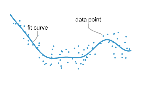
- It fits a model to the given data and displays both model and data.
- It illustrates the relationship between data and a model of the data.
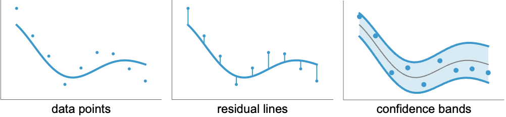
- Furthermore, it is easy to show quality measures of the fitted model such as confidence bands or residuals:
- Data values xi and yi can be given in the following forms:
-
xi a real-valued number Quantity[xi,unit] a quantity with a unit xi±ei value xi with uncertainty ei Around[xi,ei] value xi with uncertainty ei Interval[{xmin,xmax}] values between xmin and xmax - The xi and yi can also be dates, times or categorical values if appropriate settings are used for the ScalingFunctions option, or if the type information is available from the tabular data source.
- Values xi and yi that are not of the form above are taken to be missing and are not shown.
- The datai have the following forms and interpretations:
-
<"k1"y1,"k2"y2,…> values {y1,y2,…} <x1y1,x2y2,…> key-value pairs {{x1,y1},{x2,y2},…} {y1"lbl1",y2"lbl2",…}, {y1,y2,…}{"lbl1","lbl2",…} values {y1,y2,…} with labels {lbl1,lbl2,…} SparseArray values as a normal array TimeSeries, EventSeries time-value pairs QuantityArray magnitudes WeightedData unweighted values - ListFitPlot[Tabular[…]cspec] extracts and plots values from the tabular object using the column specification cspec.
- The following forms of column specifications cspec are allowed for plotting tabular data:
-
{colx,coly} plot column y against column x {{colx1,coly1},{colx2,coly2},…} plot column y1 against column x1, y2 against x2, etc. coly, {coly} plot column y as a sequence of values {{coly1},…,{colyi},…} plot columns y1, y2, etc. as sequences of values - The colx can also be Automatic, in which case sequential values are generated using DataRange.
- The following wrappers w can be used for the datai:
-
Annotation[datai,label] provide an annotation for the data Button[datai,action] define an action to execute when the data is clicked Callout[datai,label] label the data with a callout Callout[datai,label,pos] place the callout at relative position pos EventHandler[datai,events] define a general event handler for the data Highlighted[datai,effect] dynamically highlight fi with an effect Highlighted[datai,Placed[effect,pos]] statically highlight fi with an effect at position pos Hyperlink[datai,uri] make the data a hyperlink Labeled[datai,label] label the data Labeled[datai,label,pos] place the label at relative position pos Legended[datai,label] identify the data in a legend PopupWindow[datai,cont] attach a popup window to the data StatusArea[datai,label] display in the status area on mouseover Style[datai,styles] show the data using the specified styles Tooltip[datai,label] attach a tooltip to the curve - Wrappers w can be applied at multiple levels:
-
{…,w[yi],…} wrap the value yi in data {…,w[{xi,yi}],…} wrap the point {xi,yi} w[datai] wrap the data w[{data1,…}] wrap a collection of datai w1[w2[…]] use nested wrappers - Callout, Labeled and Placed can use the following positions pos:
-
Above position above curve 
Below position below curve 
Before position before curve 
After position after curve 
"Start" position at start of each curve 
"End" position at end of each curve 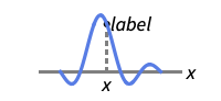
x near the curve at a position x 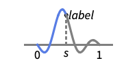
Scaled[s] scaled position s along the curve 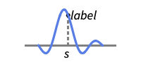
{s,Above} above relative position at position s along the curve 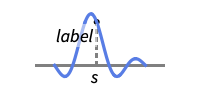
{s,Below} below relative position at position s along the curve 
{pos,epos} epos in label placed at relative position pos of the curve - ListFitPlot has the same options as Graphics, with the following additions and changes: [List of all options]
-
AspectRatio 1/GoldenRatio ratio of height to width Axes True whether to draw axes ClippingStyle None what to draw when lines are clipped ColorFunction Automatic how to determine the coloring of lines ColorFunctionScaling True whether to scale arguments to ColorFunction DataRange Automatic the range of x values to assume for data Filling None filling under each line FillingStyle Automatic style to use for filling InterpolationOrder None the polynomial degree of curves used in joining data points IntervalMarkers Automatic how to render uncertainty IntervalMarkersStyle Automatic style for uncertainty elements LabelingFunction Automatic how to label points LabelingSize Automatic maximum size of callouts and labels LabelingTarget Automatic how to determine automatic label positions MaxPlotPoints Infinity the maximum number of points to include Mesh None how many mesh points to draw on each line MeshFunctions {#1&} how to determine the placement of mesh points MeshShading None how to shade regions between mesh points MeshStyle Automatic the style for mesh points Method Automatic methods to use MultiaxisArrangement None how to arrange multiple axes for data PerformanceGoal $PerformanceGoal aspects of performance to try to optimize PlotFit Automatic how to fit a curve to the points PlotFitElements Automatic fitted elements to show in the plot PlotHighlighting Automatic highlighting effect for points PlotInteractivity $PlotInteractivity whether to allow interactive elements PlotLabel None overall label for the plot PlotLabels None labels for data PlotLayout "Overlaid" how to position data PlotLegends None legends for data PlotMarkers None markers to use to indicate each point PlotRange Automatic range of values to include PlotRangeClipping True whether to clip at the plot range PlotStyle Automatic graphics directives to determine the style of each line PlotTheme $PlotTheme overall theme for the plot ScalingFunctions None how to scale individual coordinates TargetUnits Automatic units to display in the plot - PlotFitfit determines what method is used to fit a curve to the data.
- Possible settings for fit include:
-

Automatic automatically choose the fitting model 
"Linear" use linear regression 
"Quadratic" use a quadratic model 
"Cubic" use a cubic model 
"Exponential" use an exponential model 
model use the provided FittedModel model - The simple models like "Linear" etc. all use LinearModelFit to compute the resulting fitted model.
- PlotFitElementselems controls what visual elements to include for comparing the fitted curve to the original data points.
- Possible settings for elems include:
-
None show only the fitted curve Automatic automatically chosen elements "DataPoints" show the original data "BandCurves" show 95% confidence bands "Residuals" draw residual lines between points and fitted curve {elem,<"param"value,…>} modify the parameter "param" for elem {elem1,elem2,…} combine multiple visual elements - DataRange determines how values {y1,…,yn} are interpreted into {{x1,y1},…,{xn,yn}}. Possible settings include:
-
Automatic,All uniform from 1 to n {xmin,xmax} uniform from xmin to xmax - In general, a list of pairs {{x1,y1},{x2,y2},…} is interpreted as a list of points, but the setting DataRangeAll forces it to be interpreted as multiple data sources {{y11,y12},{y21,y23},…}.
- LabelingFunction->f specifies that each point should have a label given by f[value,index,lbls], where value is the value associated with the point, index is its position in the data and lbls is the list of relevant labels.
- Possible settings for PlotLayout that show multiple curves in a single plot panel include:
-

"Overlaid" show all the data overlapping 
"Stacked" accumulate the data 
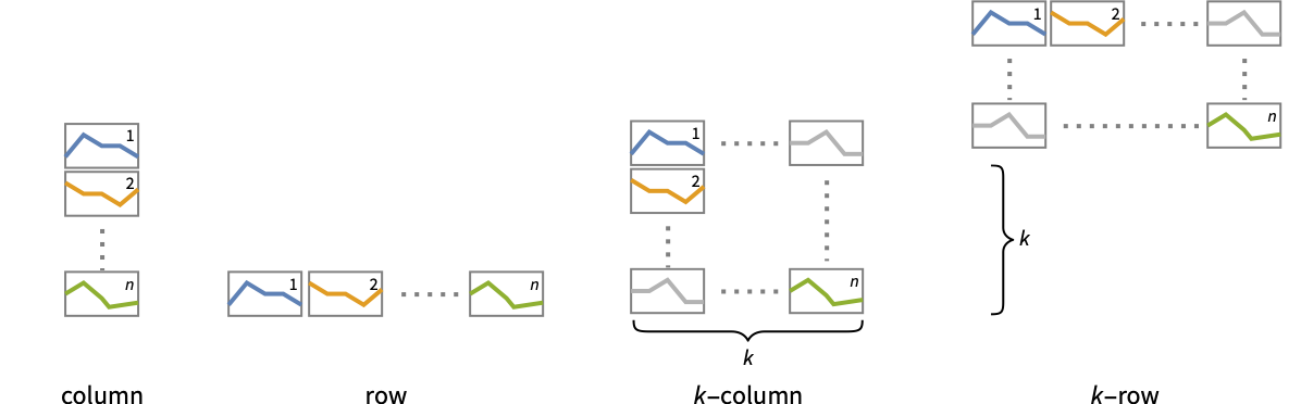
"Percentile" accumulate and normalize the data - Possible settings for PlotLayout that show single curves in multiple plot panels include:
-
"Column" use separate curves in a column of panels "Row" use separate curves in a row of panels {"Column",k},{"Row",k} use k columns or rows {"Column",UpTo[k]},{"Row",UpTo[k]} use at most k columns or rows - Possible keys and values in assoc for specifying regression parameters include:
-
"SmoothingFunction" Automatic use KernelModelFit to draw the regression line "SupportFunction" Automatic local support function to use with Automatic smoothing "GridPoints" Automatic grid points to use for the fit "Bandwidth" Automatic bandwidth to use with the smoothing function "SmoothingOptions" Automatic options for the smoothing function - Possible highlighting effects for Highlighted and PlotHighlighting include:
-
style highlight the indicated curve 
"Ball" highlight and label the indicated point in a curve 
"Dropline" highlight and label the indicated point in a curve with droplines to the axes 
"XSlice" highlight and label all points along a vertical slice 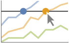
"YSlice" highlight and label all points along a horizontal slice 
Placed[effect,pos] statically highlight the given position pos - Typical settings for PlotLegends include:
-
None no legend Automatic automatically determine legend {lbl1,lbl2,…} use lbl1, lbl2, … as legend labels Placed[lspec,…] specify placement for legend - ScalingFunctions->"scale" scales the
 coordinate; ScalingFunctions{"scalex","scaley"} scales both the
  and
and  coordinates.
List of all options
Examples
open all close allBasic Examples (4)
Plot a fit curve for a list of ![]() values:
values:
ListFitPlot[AirTemperatureData[[Champaign, IL], {[Jan 1, 2024], [Dec 31, 2024], "Day"}]]Plot regression lines with automatic smoothing:
ListFitPlot[ResourceData["Sample Data: Car Stopping Distances"], AxesLabel -> Automatic]Plot a linear regression line:
ListFitPlot[ResourceData["Sample Data: Car Stopping Distances"], PlotFit -> "Linear", AxesLabel -> Automatic]Plot regression lines with 95% confidence bands:
ListFitPlot[ToTabular[ResourceData["Sample Data: Puromycin Reaction Velocity"]] -> {"Concentration", "Rate"}, PlotFitElements -> "BandCurves"]Scope (11)
General Data (3)
Plot regression lines for data including units:
ListFitPlot[ToTabular[ResourceData["Sample Data: Crab Measures"]] -> {"CarapaceLength", "BodyDepth"}, AxesLabel -> Automatic]Plot a fit curve for a sequence of ![]() ,
, ![]() pairs:
pairs:
ListFitPlot[EntityValue["Element", {"MeltingPoint", "BoilingPoint"}], PlotFitElements -> "DataPoints"]Plot multiple datasets with regression lines:
ListFitPlot[ToTabular[ResourceData["Sample Data: CPU Performance"]] -> {{"CacheSize", "PublishedPerformance"}, {"MaximumNumberOfChannels", "PublishedPerformance"}}]Tabular Data (1)
timings = Tabular[IconizedObject[«timings»], {"vertices", "edges", "connected", "edge coloring", "spanning tree", "shortest tour"}]Plot the trend line for time to compute an edge coloring for a graph against the number of vertices:
ListFitPlot[timings -> {"vertices", "edge coloring"}]Plot the trend of times in row order:
ListFitPlot[timings -> "edge coloring"]Special Data (7)
Plot a linear regression line:
ListFitPlot[{...}, PlotFit -> "Linear"]Plot a quadratic regression line:
ListFitPlot[{...}, PlotFit -> "Quadratic"]ListFitPlot[{...}, PlotFit -> "Cubic"]Plot an exponential regression line:
ListFitPlot[Last[HistogramList[RandomVariate[ExponentialDistribution[.1], 10 ^ 3]]], PlotFit -> "Exponential"]Plot 95% confidence bands along with the linear regression line:
ListFitPlot[{...}, PlotFit -> "Linear", PlotFitElements -> "BandCurves"]Plot residual lines along with the linear regression line:
ListFitPlot[{...}, PlotFit -> "Linear", PlotFitElements -> "Residuals"]Plot data points in a specified style:
ListFitPlot[{...}, PlotFit -> "Linear", PlotFitElements -> {"DataPoints", <|"Style" -> Red|>}]Options (49)
DataRange (3)
Lists of height values are displayed against the number of elements:
ListFitPlot[{...}]Rescale to the sampling space:
ListFitPlot[{...}, DataRange -> {0, 2Pi}]Each dataset is scaled to the same domain:
ListFitPlot[Table[Accumulate[RandomReal[{-1, 1}, 25]], {3}], DataRange -> {0, 1}]Filling (2)
LabelingFunction (6)
By default, points are automatically labeled with strings:
ListFitPlot[{1, 1, 2, 3, 5, 8} -> {"a", "b", "c", "d", "e", "f"}]Use LabelingFunction->None to suppress the labels:
ListFitPlot[{1, 1, 2, 3, 5, 8} -> {"a", "b", "c", "d", "e", "f"}, LabelingFunction -> None]Put the labels to the right of the points:
ListFitPlot[{1, 1, 2, 3, 5, 8} -> {"a", "b", "c", "d", "e", "f"}, LabelingFunction -> Right]Use callouts to label the points:
ListFitPlot[{1, 1, 2, 3, 5, 8} -> {"a", "b", "c", "d", "e", "f"}, LabelingFunction -> Callout[Automatic, Automatic]]Label the points with their values:
ListFitPlot[{1, 1, 2, 3, 5, 8} -> {"a", "b", "c", "d", "e", "f"}, LabelingFunction -> (#1&)]Label the points with their indices:
ListFitPlot[{1, 1, 2, 3, 5, 8} -> {"a", "b", "c", "d", "e", "f"}, LabelingFunction -> (#2&)]LabelingSize (4)
Textual labels are shown at their actual sizes:
ListFitPlot[{1, 1, 2, 3, 5, 8} -> {"healthfulness", "obstreperous", "spectrogram", "vestige", "coinage", "limey"}, ImageSize -> Medium]Image labels are automatically resized:
ListFitPlot[{1, 1, 2, 3, 5, 8} -> {[image], [image], [image], [image], [image], [image]}, ImageSize -> Medium]Specify a maximum size for textual labels:
ListFitPlot[{1, 1, 2, 3, 5, 8} -> {"healthfulness", "obstreperous", "spectrogram", "vestige", "coinage", "limey"}, ImageSize -> Medium, LabelingSize -> 30]Specify a maximum size for image labels:
ListFitPlot[{1, 1, 2, 3, 5, 8} -> {[image], [image], [image], [image], [image], [image]}, ImageSize -> Medium, LabelingSize -> 20]Show image labels at their natural sizes:
ListFitPlot[{1, 1, 2, 3, 5, 8} -> {[image], [image], [image], [image], [image], [image]}, ImageSize -> Medium, LabelingSize -> Full]LabelingTarget (6)
Labels are automatically placed to maximize readability:
ListFitPlot[IconizedObject[«data»]]ListFitPlot[IconizedObject[«data»], LabelingTarget -> All]Use a denser layout for the labels:
ListFitPlot[IconizedObject[«data»], LabelingTarget -> "Dense"]Show the quarter of the labels that are easiest to read:
ListFitPlot[IconizedObject[«data»], LabelingTarget -> 0.25]Only allow labels that are orthogonal to the points:
ListFitPlot[IconizedObject[«data»], LabelingTarget -> <|"AllowedLabelingPositions" -> "Sides"|>]Only allow labels that are diagonal to the points:
ListFitPlot[IconizedObject[«data»], LabelingTarget -> <|"AllowedLabelingPositions" -> "Corners"|>]Restrict labels to be above or to the right of the points:
ListFitPlot[IconizedObject[«data»], LabelingTarget -> <|"AllowedLabelingPositions" -> {"Right", "Top"}|>]Allow labels to be clipped by the edges of the plot:
ListFitPlot[IconizedObject[«data»], LabelingTarget -> <|"AllowLabelClipping" -> True|>]IntervalMarkers (2)
IntervalMarkersStyle (2)
Uncertainties automatically inherit the plot style:
ListFitPlot[{Table[Around[RandomReal[20], 1], 10], Table[Around[RandomReal[20], 1], 10]}, PlotStyle -> {Red, Blue}]Specify the style for uncertainties:
ListFitPlot[{Table[Around[RandomReal[20], 1], 10], Table[Around[RandomReal[20], 1], 10]}, IntervalMarkersStyle -> Gray]MultiaxisArrangement (5)
By default, all items in a plot share the same scale:
ListFitPlot[{RandomInteger[100, 10], Prime[RandomInteger[200, 10]]}]Use different axes for the different items:
ListFitPlot[{RandomInteger[100, 10], Prime[RandomInteger[200, 10]]}, MultiaxisArrangement -> All]Any number of axes can be used:
ListFitPlot[{RandomInteger[100, 10], Prime[RandomInteger[200, 10]], RandomInteger[10, 10] ^ 2}, MultiaxisArrangement -> All]Have the first and second curves share an axis:
ListFitPlot[{RandomInteger[100, 10], Prime[RandomInteger[200, 10]], RandomInteger[10, 10] ^ 2}, MultiaxisArrangement -> {{1, 2}, 3}]Specify where the axes should be placed:
ListFitPlot[{RandomInteger[100, 10], Prime[RandomInteger[200, 10]], RandomInteger[10, 10] ^ 2}, MultiaxisArrangement -> {Right -> {1, 2}, Left -> 3}]ListFitPlot[{RandomInteger[100, 10], Prime[RandomInteger[200, 10]], RandomInteger[10, 10] ^ 2}, MultiaxisArrangement -> {Right -> {{1, 2}}, Left -> 3}]PlotFit (4)
Automatically fit a model to the data:
ListFitPlot[ResourceData["Sample Tabular Data: Car Models"] -> {"mpg", "weight"}]Fit a straight line to the data:
ListFitPlot[ResourceData["Sample Tabular Data: Car Models"] -> {"mpg", "weight"}, PlotFit -> "Linear"]Fit a quadratic curve to the data:
ListFitPlot[ResourceData["Sample Tabular Data: Car Models"] -> {"mpg", "weight"}, PlotFit -> "Quadratic"]Use KernelModelFit to approximate the data:
ListFitPlot[ResourceData["Sample Tabular Data: Car Models"] -> {"mpg", "weight"}, PlotFit -> "Kernel"]PlotFitElements (3)
By default, the fitted model is shown with the data points:
ListFitPlot[ResourceData["Sample Tabular Data: Car Models"] -> {"mpg", "weight"}]Plot confidence bands for the data, with a default confidence level of 0.95:
ListFitPlot[ResourceData["Sample Tabular Data: Car Models"] -> {"mpg", "weight"}, PlotFitElements -> "BandCurves"]Use a confidence level of 0.5 for the bands:
ListFitPlot[ResourceData["Sample Tabular Data: Car Models"] -> {"mpg", "weight"}, PlotFitElements -> {"BandCurves", <|"ConfidenceLevel" -> 0.5|>}]Show residual lines from the data points to the fitted curve:
ListFitPlot[ResourceData["Sample Tabular Data: Car Models"] -> {"mpg", "weight"}, PlotFitElements -> "Residuals"]Combine the original points with gray residual lines:
ListFitPlot[ResourceData["Sample Tabular Data: Car Models"] -> {"mpg", "weight"}, PlotFitElements -> {"DataPoints", {"Residuals", <|"Style" -> Gray|>}}]PlotInteractivity (2)
PlotLayout (3)
By default, curves are overlaid on each other:
data = {{10, 9, 4, 3, 5, 3, 5, 5, 2, 6}, {2, 10, 5, 6, 9, 4, 9, 3, 7, 2}, {7, 8, 3, 4, 4, 2, 6, 3, 8, 7}};ListFitPlot[data]Plot the data in a stacked layout:
ListFitPlot[data, PlotLayout -> "Stacked"]Plot the data as percentiles of the total of the values:
ListFitPlot[data, PlotLayout -> "Percentile"]Place each curve in a separate panel using shared axes:
ListFitPlot[data, PlotLayout -> "Column", ImageSize -> Medium]ListFitPlot[data, PlotLayout -> "Row", ImageSize -> Medium]ListFitPlot[IconizedObject[«data»], ImageSize -> Medium, Joined -> True, PlotLayout -> {"Column", 4}]ListFitPlot[IconizedObject[«data»], ImageSize -> Medium, Joined -> True, PlotLayout -> {"Column", UpTo[4]}]ListFitPlot[{{...}, {...}}, Joined -> True, PlotLayout -> "Column", ImageSize -> Medium, PlotLabels -> {"First", "Second"}]PlotStyle (3)
Use different style directives:
data = Table[{i, Sin[2i] + i RandomReal[0.25] + 1}, {i, 0, 8, 0.1}];Table[ListFitPlot[data, PlotStyle -> ps], {ps, {Red, Thick, Dashed}}]By default, different styles are chosen for multiple curves:
ListFitPlot[Table[Accumulate[RandomReal[{-1, 1}, 25]], {3}]]Explicitly specify the styles for different curves:
ListFitPlot[Table[Accumulate[RandomReal[{-1, 1}, 25]], {3}], PlotStyle -> {Red, Automatic, Green, Automatic, Blue}]ScalingFunctions (2)
By default, plots have linear scales in each direction:
data = {...};ListFitPlot[data]Use a log scale in the ![]() direction:
direction:
ListFitPlot[data, ScalingFunctions -> "Log"]Use a linear scale in the ![]() direction that shows smaller numbers at the top:
direction that shows smaller numbers at the top:
ListFitPlot[data, ScalingFunctions -> "Reverse"]DateScale ticks are used automatically for TimeSeries data:
aapl = FinancialData["AAPL", {{2021, 1, 1}, {2021, 6, 1}}]ListFitPlot[aapl]Text
Wolfram Research (2025), ListFitPlot, Wolfram Language function, https://reference.wolfram.com/language/ref/ListFitPlot.html.
CMS
Wolfram Language. 2025. "ListFitPlot." Wolfram Language & System Documentation Center. Wolfram Research. https://reference.wolfram.com/language/ref/ListFitPlot.html.
APA
Wolfram Language. (2025). ListFitPlot. Wolfram Language & System Documentation Center. Retrieved from https://reference.wolfram.com/language/ref/ListFitPlot.html