


Histogram
Histogram[{x1,x2,…}]
plots a histogram of the values xi.
Histogram[{x1,x2,…},bspec]
plots a histogram with bin width specification bspec.
Histogram[{x1,x2,…},bspec,hspec]
plots a histogram with bin heights computed according to the specification hspec.
Histogram[{data1,data2,…},…]
plots histograms for multiple datasets datai.
Details and Options
- Histogram[data] by default plots a histogram with equal bin widths chosen to approximate an assumed underlying smooth distribution of the values xi.
- Data values xi can be given in the following forms:
-
xi a number Quantity[xi,unit] a number with a unit - Datasets datai have the following forms and interpretations:
-
{x1,x2,…} a list of values xi <k1x1,k2x2,…> the values xi from the association QuantityArray the magnitudes TimeSeries,EventSeries,… the values from time series data WeightedData the count for each value is its weight w[datai] wrapper w for dataset datai - Histogram[objcspec] extracts and plots values from the Tabular, TimeSeries or EventSeries object obj using the column specification cspec.
- The following specifications cspec are allowed for plotting tabular data:
-
col histogram values from key col {col1,col2,…} histogram values from keys col1,col2,… - The following bin width specifications bspec can be given:
-
n use n bins {dx} use bins of width dx {xmin,xmax,dx} use bins of width dx from xmin to xmax {{b1,b2,…}} use the bins [b1,b2),[b2,b3),… Automatic determine bin widths automatically "name" use a named binning method {"Log",bspec} apply binning bspec on log-transformed data fb apply fb to get an explicit bin specification {b1,b2,…} - The binning specification "Log" is taken to use the Automatic underlying binning method.
- Possible named binning methods include:
-
"Sturges" compute the number of bins based on the length of data "Scott" asymptotically minimize the mean square error "FreedmanDiaconis" twice the interquartile range divided by the cube root of sample size "Knuth" balance likelihood and prior probability of a piecewise uniform model "Wand" one-level recursive approximate Wand binning - The function fb in Histogram[data,fb] is applied to a list of all xi, and should return an explicit bin list {b1,b2,…}.
- Different forms of histogram can be obtained by giving different bin height specifications hspec in Histogram[data,bspec,hspec]. The following forms can be used:
-
"Count" number of elements in each bin "CumulativeCount" cumulative counts "SurvivalCount" survival counts "Probability" fraction of values lying in each bin "Intensity" count divided by bin width "PDF" probability density function "CDF" cumulative distribution function "SF" survival function "HF" hazard function "CHF" cumulative hazard function {"Log",hspec} log-transformed height specification fh heights obtained by applying fh to bins and counts - The function fh in Histogram[data,bspec,fh] is applied to two arguments: a list of bins {{b1,b2},{b2,b3},…}, and a corresponding list of counts {c1,c2,…}. The function should return a list of heights to be used for each of the ci.
- Only values xi that are real numbers are assigned to bins; others are taken to be missing.
- In Histogram[{data1,data2,…},…], automatic bin locations are determined by combining all the datasets datai.
- Histogram[{…,wi[datai,…],…},…] renders the histogram elements associated with dataset datai according to the specification defined by the symbolic wrapper wi.
- The following wrappers can be used for chart elements:
-
Annotation[e,label] provide an annotation Button[e,action] define an action to execute when the element is clicked Callout[e,label] display the element with a callout EventHandler[e,…] define a general event handler for the element Hyperlink[e,uri] make the element act as a hyperlink Labeled[e,…] display the element with labeling Legended[e,…] include features of the element in a chart legend Mouseover[e,over] make the element show a mouseover form PopupWindow[e,cont] attach a popup window to the element StatusArea[e,label] display in the status area when the element is moused over Style[e,opts] show the element using the specified styles Tooltip[e,label] attach an arbitrary tooltip to the element - Histogram has the same options as Graphics with the following additions and changes: [List of all options]
-
AspectRatio 1/GoldenRatio ratio of height to width Axes True whether to draw axes BarOrigin Bottom origin of histogram bars ChartElementFunction Automatic how to generate raw graphics for bars ChartElements Automatic graphics to use in each of the bars ColorFunction Automatic how to color bars ColorFunctionScaling True whether to normalize arguments to ColorFunction LabelingFunction Automatic how to label elements LegendAppearance Automatic overall appearance of legends PerformanceGoal $PerformanceGoal aspects of performance to try to optimize PlotFit None how to fit a curve to the histogram PlotFitElements Automatic fitted elements to show in the histogram PlotInteractivity $PlotInteractivity whether to allow interactive elements PlotLabels None category labels for datasets PlotLayout Automatic overall layout to use PlotLegends None legends for data elements and datasets PlotStyle Automatic style for bars PlotTheme $PlotTheme overall theme for the histogram ScalingFunctions None how to scale individual coordinates TargetUnits Automatic units to display in the chart - The following settings for PlotLayout can be used to display multiple sets of data:
-
"Overlapped" show all the data overlapping 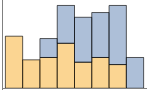
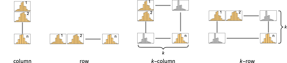
"Stacked" accumulate the data per bin - Possible settings for PlotLayout that show single groups of bars in multiple panels include:
-
"Column" use separate groups of bars in a column of panels "Row" use separate groups of bars in a row of panels {"Column",k},{"Row",k} use k columns or rows {"Column",UpTo[k]},{"Row",UpTo[k]} use at most k columns or rows - Typical settings for PlotLegends include:
-
None no legend Automatic automatically determine legend {lbl1,lbl2,…} use lbl1, lbl2, … as legend labels Placed[lspec,…] specify placement for legend - PlotStylesty specifies the styles to use for each curve. Possible settings include:
-
{sty1,sty2,…} sequence of styles for the datasets <"key"val,…> styling elements for different levels of data - The accepted keys are:
-
"Base" overall style for all the datai "Lists" list of styles styi for each datai - ColorData["DefaultChartColors"] gives the default sequence of colors used by PlotStyle.
- The arguments supplied to ChartElementFunction are the bin region {{xmin,xmax},{ymin,ymax}}, the bin values lists, and metadata {m1,m2,…} from each level in a nested list of datasets.
- A list of built-in settings for ChartElementFunction can be obtained from ChartElementData["Histogram"].
- The argument supplied to ColorFunction is the height for each bin.
- With ScalingFunctions->{sx,sy}, the
 coordinate is scaled using sx etc.
 - Style and other specifications from options and other constructs in BarChart are effectively applied in the order PlotStyle, ColorFunction, Style and other wrappers, ChartElements and ChartElementFunction, with later specifications overriding earlier ones.
List of all options
Examples
open all close allBasic Examples (4)
Generate a histogram for a list of values:
Histogram[RandomVariate[NormalDistribution[0, 1], 200]]data1 = RandomVariate[NormalDistribution[0, 1], 500];
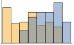
data2 = RandomVariate[NormalDistribution[3, 1 / 2], 500];Histogram[{data1, data2}]Generate a probability histogram for a list of values:
Histogram[RandomVariate[WeibullDistribution[2, 1], 1000], Automatic, "Probability"]Show multiple datasets as a row of individual histograms:
Histogram[{IconizedObject[«data1»], IconizedObject[«data2»]}, PlotLayout -> "Row"]Scope (35)
Data and Layouts (19)
Specify the number of bins to use:
data = RandomVariate[NormalDistribution[0, 1], 200];Histogram[data, 5]Histogram[data, {.5}]Histogram[data, {-2, 2, 1}]The bin delimiters as an explicit list:
Histogram[data, {{-3, -1, 0, 1, 3}}]Bins for discrete values are centered over the values when possible:
Histogram[RandomInteger[10, 250]]Use different automatic binning methods:
data = RandomVariate[NormalDistribution[0, 1], 1000];Table[Histogram[data, b, PlotLabel -> b], {b, {"Sturges", "Scott", "FreedmanDiaconis", "Wand"}}]Use logarithmically spaced bins:
Histogram[data, "Log"]Delimit bins on integer boundaries using a binning function:
integerBins[list_] := Union[IntegerPart[list]]integerBins[{1.2, 1.8, 2.3, 2.5}]Histogram[RandomReal[20, 100], integerBins]Use different height specifications:
data = RandomVariate[NormalDistribution[0, 1], 200];Table[Histogram[data, Automatic, h, PlotLabel -> h], {h, {"Count", "Probability", "PDF", "CumulativeCount", "CDF", "SF"}}]Use a height function that accumulates the bin counts:
accumulatedCount[bins_, counts_] := Accumulate[counts]Histogram[RandomVariate[NormalDistribution[0, 1], 200], Automatic, accumulatedCount]Bins associated with a dataset are styled the same:
data1 = RandomVariate[NormalDistribution[0, 1], 500];
data2 = RandomVariate[NormalDistribution[3, 1 / 2], 500];
data3 = RandomVariate[NormalDistribution[5, 1 / 3], 500];Histogram[{data1, data2, data3}]Nonreal data is taken to be missing:
Histogram[{1, 2, 3, None, 3, 5, Missing[], 2, 1, foo, 2, 3}]data1 = RandomVariate[NormalDistribution[0, 1], 500];
data2 = RandomVariate[NormalDistribution[3, 1 / 2], 500];Histogram[{data1, None, data2}]Histogram[{Quantity[1, "Meters"], Quantity[3, "Meters"], Quantity[2, "Meters"], Quantity[2, "Meters"], Quantity[3, "Meters"], Quantity[2, "Meters"], Quantity[5, "Meters"], Quantity[3, "Meters"], Quantity[2, "Meters"], Quantity[4, "Meters"]}, AxesLabel -> Automatic]Histogram[{Quantity[1, "Meters"], Quantity[3, "Meters"], Quantity[2, "Meters"], Quantity[2, "Meters"], Quantity[3, "Meters"], Quantity[2, "Meters"], Quantity[5, "Meters"], Quantity[3, "Meters"], Quantity[2, "Meters"], Quantity[4, "Meters"]}, AxesLabel -> Automatic, TargetUnits -> "Feet"]Specify binning spec with units:
Histogram[{Quantity[6, "Meters"], Quantity[6, "Meters"], Quantity[9, "Meters"], Quantity[2, "Meters"], Quantity[9, "Meters"], Quantity[8, "Meters"], Quantity[9, "Meters"], Quantity[5, "Meters"], Quantity[2, "Meters"], Quantity[6, "Meters"], Quantity[5, "Meters"], Quantity[10, "Meters"], Quantity[7, "Meters"], Quantity[9, "Meters"], Quantity[10, "Meters"], Quantity[3, "Meters"], Quantity[8, "Meters"], Quantity[3, "Meters"], Quantity[2, "Meters"], Quantity[1, "Meters"], Quantity[7, "Meters"], Quantity[2, "Meters"], Quantity[7, "Meters"], Quantity[5, "Meters"], Quantity[4, "Meters"]}, {Quantity[0, "Feet"], Quantity[20, "Feet"], Quantity[4, "Feet"]}, AxesLabel -> Automatic]The values in an association are used as elements:
Histogram[<|"a" -> 2, "b" -> 3, "c" -> 5, "d" -> 7, "e" -> 11, "f" -> 13|>, 5]Histogram[<|"data one" -> <|"a" -> 6, "b" -> 3, "c" -> 5, "d" -> 7, "e" -> 11, "f" -> 13|>, "data two" -> <|"a" -> 26, "b" -> 23, "c" -> 32, "d" -> 29, "e" -> 21, "f" -> 38|>|>, 6]Histogram[<|"data one" -> {6, 3, 5, 7, 11, 13}, "data two" -> {26, 23, 32, 29, 21, 38}|>, 6, PlotLabels -> Automatic]Histogram[<|"data one" -> {6, 3, 5, 7, 11, 13}, "data two" -> {26, 23, 32, 29, 21, 38}|>, 6, PlotLegends -> Automatic]The time stamps in TimeSeries, EventSeries, and TemporalData are ignored:
data = RandomVariate[NormalDistribution[], 50];{Histogram[data], Histogram[TimeSeries[data, {"May 24, 1982"}]]}Weights in WeightedData affect the shape of histogram:
data = RandomInteger[{1, 25}, 5000];{Histogram[data], Histogram[data, Automatic, "PDF"]}wd = WeightedData[data, Function@@{t, t^2}];{Histogram[wd], Histogram[wd, Automatic, "PDF"]}The censoring and truncation information in EventData also affects the histogram:
data = RandomVariate[WeibullDistribution[3, 4], 200];
t = Table[If[i > 4, 4, i], {i, data}];
c = Table[Boole[i == 4], {i, t}];𝒜 = EventData[t, c]{Histogram[data, Automatic, "PDF"], Histogram[𝒜, Automatic, "PDF"]}Use different layouts to display multiple datasets:
data1 = RandomVariate[NormalDistribution[0, 1], 500];
data2 = RandomVariate[NormalDistribution[0, 1], 500];Table[Histogram[{data1, data2}, PlotLabel -> l, ChartLayout -> l], {l, {"Overlapped", "Stacked"}}]Use rows and columns of individual plots to show multiple sets:
data1 = RandomVariate[NormalDistribution[0, 1], 500];
data2 = RandomVariate[NormalDistribution[0, 2], 500];Histogram[{data1, data2}, ChartLayout -> "Row"]Histogram[{data1, data2}, ChartLayout -> "Column"]Table[Histogram[RandomVariate[NormalDistribution[0, 1], 200], BarOrigin -> o, PlotLabel -> o, Ticks -> None], {o, {Bottom, Left, Top, Right}}]Tabular Data (3)
tabular = Tabular[ExampleData[{"Statistics", "USCars1993"}], ExampleData[{"Statistics", "USCars1993"}, "ColumnHeadings"]]Generate a histogram for city mileage:
Histogram[tabular -> "MPGcity"]Create overlaid histograms for city and highway mileage:
Histogram[tabular -> {"MPGcity", "MPGhighway"}]Use smaller bin sizes for the data:
Histogram[tabular -> {"MPGcity", "MPGhighway"}, {1}]View the distributions side by side:
Histogram[tabular -> {"MPGcity", "MPGhighway"}, {1}, ChartLayout -> "Row"]Histogram the values for all the components in TimeSeries or EventSeries:
Histogram[TimeSeries[TimeEventSeries`TimestampData[Association["UniformlySpacedQ" -> False,
"Timestamps" -> TabularColumn[Association[
"Data" -> {363, {{NumericArray[{19723, 19724, 19725, 19726, 19727, 19728, 19729, 19730,
19731, 19732, ... ///3///////////3///f/zv/////w=="],
"Capacity" -> 363, "BitCount" -> 352}] -> Missing["Unmatched"]},
"ElementType" -> TypeSpecifier["Quantity"]["NumberExpression",
"DegreesCelsius"]]]}}]]]], Association[]]]Histogram the values for a component of a TimeSeries or EventSeries:
temps = TimeSeries[TimeEventSeries`TimestampData[Association["UniformlySpacedQ" -> False,
"Timestamps" -> TabularColumn[Association[
"Data" -> {363, {{NumericArray[{19723, 19724, 19725, 19726, 19727, 19728, 19729, 19730,
19731, 19732, ... ///3///////////3///f/zv/////w=="],
"Capacity" -> 363, "BitCount" -> 352}] -> Missing["Unmatched"]},
"ElementType" -> TypeSpecifier["Quantity"]["NumberExpression",
"DegreesCelsius"]]]}}]]]], Association[]];Histogram[temps -> "Champaign"]Histogram values from multiple components:
Histogram[temps -> {"Oxford", "Tokyo"}, PlotLegends -> {"Oxford", "Tokyo"}]Wrappers (2)
Use wrappers on individual data, datasets, or collections of datasets:
data1 = RandomVariate[NormalDistribution[0, 1], 500];
data2 = RandomVariate[NormalDistribution[3, 1 / 2], 500];
data3 = RandomVariate[NormalDistribution[5, 1 / 3], 500];{Histogram[{data1, data2, data3}], Histogram[{data1, Style[data2, RGBColor[0.14, 0.8, 0.14]], data3}], Histogram[Style[{data1, data2, data3}, RGBColor[0.14, 0.8, 0.14]]]}Histogram[Style[{data1, Style[data2, RGBColor[0.14, 0.8, 0.14]], data3}, RGBColor[1, 0.75, 0]]]Override the default tooltips:
data1 = RandomVariate[NormalDistribution[0, 1], 500];
data2 = RandomVariate[NormalDistribution[3, 1 / 2], 500];
data3 = RandomVariate[NormalDistribution[5, 1 / 3], 500];Histogram[{data1, Tooltip[data2, "my data"], data3}]Use PopupWindow to provide additional drilldown information:
Histogram[{data1, PopupWindow[data2, DateListPlot[FinancialData["IBM", "Jan. 1, 2004"]]], data3}]Button can be used to trigger any action:
Histogram[{data1, Button[data2, Speak["my data"]], data3}]Styling and Appearance (4)
Use an explicit list of styles for the bars:
data1 = RandomVariate[NormalDistribution[0, 1], 500];
data2 = RandomVariate[NormalDistribution[3, 1 / 2], 500];
data3 = RandomVariate[NormalDistribution[5, 1 / 3], 500];Histogram[{data1, data2, data3}, PlotStyle -> {RGBColor[0.93, 0.27, 0.27], RGBColor[0.14, 0.8, 0.14], RGBColor[0.4, 0.6, 1]}]Style can be used to override styles:
Histogram[{data1, Style[data2, RGBColor[0.93, 0.27, 0.27]], data3}, PlotStyle -> GrayLevel[0.62]]Use any graphic for pictorial bars:
Histogram[RandomVariate[NormalDistribution[0, 1], 500], ChartElements -> Graphics[Disk[]]]Use built-in, programmatically generated bars:
ChartElementData["Histogram"]Table[Histogram[RandomVariate[NormalDistribution[0, 1], 200], ChartElementFunction -> f], {f, {"GlassRectangle", "GradientScaleRectangle"}}]For detailed settings, use Palettes ▶ ChartElementSchemes:
Histogram[RandomVariate[NormalDistribution[0, 1], 200], ChartElementFunction -> ChartElementDataFunction["SegmentScaleRectangle", "Segments" -> 7, "ColorScheme" -> "SolarColors"]]Histogram[Table[RandomVariate[NormalDistribution[i, 0.93 ^ i], 1000], {i, {0, 3, 6, 9}}], 50, PlotTheme -> "Monochrome"]Labeling and Legending (7)
Use Labeled to add a label to a dataset:
data1 = RandomVariate[NormalDistribution[0, 1], 500];
data2 = RandomVariate[NormalDistribution[3, 1 / 2], 500];
data3 = RandomVariate[NormalDistribution[5, 1 / 3], 500];Histogram[{data1, data2, Labeled[data3, "label", Above]}]Use symbolic positions for label placement:
Table[Histogram[Labeled[RandomVariate[NormalDistribution[0, 1], 500], "label", p], PlotLabel -> p], {p, {Bottom, Center, Top}}]Table[Histogram[Labeled[RandomVariate[NormalDistribution[0, 1], 500], "label", p], PlotLabel -> p], {p, {Left, Center, Right}}]Provide value labels for bars by using LabelingFunction:
Histogram[RandomVariate[NormalDistribution[0, 1], 500], LabelingFunction -> Above]Use Placed to control placement and formatting:
labeler[v_, {i_, j_}, {ri_, cj_}] := Placed[{CharacterRange["A", "Z"][[j]], v}, Above, Column]Histogram[RandomVariate[NormalDistribution[0, 1], 500], LabelingFunction -> labeler]Add categorical legend entries for datasets:
data1 = RandomVariate[NormalDistribution[0, 1], 500];
data2 = RandomVariate[NormalDistribution[3, 1 / 2], 500];
data3 = RandomVariate[NormalDistribution[5, 1 / 3], 500];Histogram[{data1, data2, data3}, PlotLegends -> {"ccc1", "ccc2", "ccc3"}]Use Legended to add additional legend entries:
data1 = RandomVariate[NormalDistribution[0, 1], 500];
data2 = RandomVariate[NormalDistribution[3, 1 / 2], 500];
data3 = RandomVariate[NormalDistribution[5, 1 / 3], 500];Histogram[{data1, Legended[Style[data2, RGBColor[0.93, 0.27, 0.27]], "extra"], data3}, PlotLegends -> {"aaa", "bbb", "ccc"}]Use Placed to affect the positioning of legends:
data1 = RandomVariate[NormalDistribution[0, 1], 500];
data2 = RandomVariate[NormalDistribution[3, 1 / 2], 500];
data3 = RandomVariate[NormalDistribution[5, 1 / 3], 500];Table[Histogram[{data1, data2, data3}, PlotLegends -> Placed[{"ccc1", "ccc2", "ccc3"}, p]], {p, {Below, Above}}]Options (89)
AspectRatio (3)
By default, Histogram uses a fixed height to width ratio for the plot:
Histogram[IconizedObject[«random data»]]Make the height the same as the width with AspectRatio1:
Histogram[IconizedObject[«random data»], AspectRatio -> 1]AspectRatioFull adjusts the height and width to tightly fit inside other constructs:
plot = Histogram[IconizedObject[«random data»], AspectRatio -> Full];{Framed[Pane[plot, {50, 100}]], Framed[Pane[plot, {100, 100}]], Framed[Pane[plot, {100, 75}]]}Axes (4)
By default, Axes are drawn:
Histogram[IconizedObject[«random data»]]Use AxesFalse to turn off axes:
Histogram[IconizedObject[«random data»], Axes -> False]Use AxesOrigin to specify where the axes intersect:
Histogram[IconizedObject[«random data»], AxesOrigin -> {0, 0}]Turn each axis on individually:
{Histogram[IconizedObject[«random data»], Axes -> {True, False}], Histogram[IconizedObject[«random data»], Axes -> {False, True}]}AxesLabel (4)
No axes labels are drawn by default:
Histogram[IconizedObject[«random data»]]Histogram[IconizedObject[«random data»], AxesLabel -> y]Histogram[IconizedObject[«random data»], AxesLabel -> {x, n}]Histogram[QuantityArray[IconizedObject[«random data»], "Meters"], AxesLabel -> Automatic]AxesOrigin (2)
AxesStyle (4)
Change the style for the axes:
Histogram[IconizedObject[«random data»], AxesStyle -> RGBColor[0.93, 0.27, 0.27]]Specify the style of each axis:
Histogram[IconizedObject[«random data»], AxesStyle -> {RGBColor[0.93, 0.27, 0.27], RGBColor[0.4, 0.6, 1]}]Use different styles for the ticks and the axes:
Histogram[IconizedObject[«random data»], AxesStyle -> RGBColor[0.14, 0.8, 0.14], TicksStyle -> RGBColor[0.93, 0.27, 0.27]]Use different styles for the labels and the axes:
Histogram[IconizedObject[«random data»], AxesStyle -> RGBColor[0.14, 0.8, 0.14], LabelStyle -> RGBColor[0.93, 0.27, 0.27]]BarOrigin (1)
ChartElementFunction (5)
Get a list of built-in settings for ChartElementFunction:
ChartElementData["Histogram"]For detailed settings, use Palettes ▶ ChartElementSchemes:
data = RandomVariate[NormalDistribution[0, 1], 200];Table[Histogram[data, ChartElementFunction -> f, PlotLabel -> f], {f, {"Rectangle", "GradientRectangle"}}]Table[Histogram[data, ChartElementFunction -> f, PlotLabel -> f], {f, {"FadingRectangle", "GlassRectangle"}}]ChartElementFunction is appropriate to show the global scale:
Table[Histogram[data, ChartElementFunction -> f, PlotLabel -> f], {f, {"GradientScaleRectangle", "SegmentScaleRectangle"}}]Write a custom ChartElementFunction:
f[{{xmin_, xmax_}, {ymin_, ymax_}}, ___] := Rectangle[{xmin, ymin}, {xmax, ymax}]Histogram[RandomVariate[NormalDistribution[0, 1], 200], ChartElementFunction -> f]g[{{xmin_, xmax_}, {ymin_, ymax_}}, ___] := Polygon[{{xmin, ymin}, {xmax, ymax}, {xmin, ymax}, {xmax, ymin}}]Histogram[RandomVariate[NormalDistribution[0, 1], 200], ChartElementFunction -> g]Use metadata passed on from the input, in this case charting the data:
DataDrilldownBar[{{xmin_, xmax_}, {ymin_, ymax_}}, data_, {True}, ___] :=
PopupWindow[Polygon[{{xmin, ymin}, {xmax, ymax}, {xmin, ymax}, {xmax, ymin}}], PieChart[data]]DataDrilldownBar[{{xmin_, xmax_}, {ymin_, ymax_}}, ___] :=
Rectangle[{xmin, ymin}, {xmax, ymax}]data1 = RandomVariate[NormalDistribution[0, 1], 500];
data2 = RandomVariate[NormalDistribution[3, 1 / 2], 500];
data3 = RandomVariate[NormalDistribution[5, 1 / 3], 500];Histogram[{data1, data2 -> True, data3}, ChartElementFunction -> DataDrilldownBar]Built-in element functions may have options; use Palettes ▶ ChartElementSchemes to set them:
ChartElementData["Rectangle", "Options"]data = RandomVariate[NormalDistribution[0, 1], 500];Table[Histogram[data, ChartElementFunction -> ChartElementData["Rectangle", "RoundingRadius" -> r], PlotLabel -> r], {r, {0, 3, 6}}]ChartElements (9)
Create a pictorial chart based on any Graphics object:
Histogram[RandomVariate[NormalDistribution[0, 1], 200], ChartElements -> Graphics[Disk[]]]Histogram[RandomVariate[NormalDistribution[0, 1], 50], ChartElements -> Graphics3D[Sphere[]]]Histogram[RandomVariate[NormalDistribution[0, 1], 50], ChartElements -> ExampleData[{"TestImage", "House"}]]Use a stretched version of the graphic:
Histogram[RandomVariate[NormalDistribution[0, 1], 200], ChartElements -> {[image], All}]Use explicit sizes for width and height:
data = RandomVariate[NormalDistribution[0, 1], 100];Table[Histogram[data, ChartElements -> {Graphics[Disk[], AspectRatio -> Full], s}, PlotLabel -> s], {s, {{1 / 2, 5}, {1, 3}}}]Using All for width or height causes that direction to stretch to the full size of the bar:
data = RandomVariate[NormalDistribution[0, 1], 100];Table[Histogram[data, ChartElements -> {[image], s}, PlotLabel -> s], {s, {{1 / 2, All}, {All, 20}}}]Use a different graphic for each row of data:
data1 = RandomVariate[NormalDistribution[0, 1], 500];
data2 = RandomVariate[NormalDistribution[3, 1 / 2], 500];
data3 = RandomVariate[NormalDistribution[5, 1 / 3], 500];Histogram[{data1, data2, data3}, ChartElements -> {[image], [image], [image]}]Histogram[{data1, data2, data3}, ChartElements -> {{[image], [image]}, None}]Styles are inherited from styles set through PlotStyle etc:
Histogram[RandomVariate[NormalDistribution[0, 1], 500], ChartElements -> [image], PlotStyle -> RGBColor[0.14, 0.8, 0.14]]Style can override the settings from PlotStyle:
data1 = RandomVariate[NormalDistribution[0, 1], 500];
data2 = RandomVariate[NormalDistribution[3, 1 / 2], 500];
data3 = RandomVariate[NormalDistribution[5, 1 / 3], 500];Histogram[{data1, Style[data2, GrayLevel[0]], data3}, ChartElements -> [image], PlotStyle -> {RGBColor[0.93, 0.27, 0.27], RGBColor[0.14, 0.8, 0.14], RGBColor[0.4, 0.6, 1]}]Explicit styles set in the graphic will override other style settings:
Histogram[RandomVariate[NormalDistribution[0, 1], 500], ChartElements -> [image], PlotStyle -> RGBColor[0.14, 0.8, 0.14]]g = Graphics3D[{EdgeForm[], Specularity[White, 30], Cylinder[]}, ViewPoint -> {0, -Infinity, 0}, Boxed -> False, Lighting -> "Neutral", PlotRangePadding -> 0];Histogram[RandomVariate[NormalDistribution[0, 1], 200], ChartElements -> {g, All}, PlotStyle -> RGBColor[0.8, 0.3, 0.8]]ChartLayout (5)
Use different layouts to display multiple datasets:
data1 = RandomVariate[NormalDistribution[0, 1], 500];
data2 = RandomVariate[NormalDistribution[0, 1], 500];Table[Histogram[{data1, data2}, ChartLayout -> l, PlotLabel -> l], {l, {"Overlapped", "Stacked"}}]With multiple datasets that are fairly disjoint, typically "Overlapped" works better:
data1 = RandomVariate[NormalDistribution[0, 1], 500];
data2 = RandomVariate[NormalDistribution[3, 1], 500];Table[Histogram[{data1, data2}, ChartLayout -> l, PlotLabel -> l], {l, {"Overlapped", "Stacked"}}]Place each group of bars in a separate panel using shared axes:
Histogram[{IconizedObject[«σ = 1»], IconizedObject[«σ = 2»]}, ChartLayout -> Column]Use a row instead of a column:
Histogram[{IconizedObject[«σ = 1»], IconizedObject[«σ = 2»]}, ImageSize -> Medium, ChartLayout -> Row]Histogram[{IconizedObject[«σ = 1»], IconizedObject[«σ = 2»], IconizedObject[«σ = 3»], IconizedObject[«σ = 4»]}, ImageSize -> Medium, ChartLayout -> {"Column", 2}]Histogram[{IconizedObject[«σ = 1»], IconizedObject[«σ = 2»], IconizedObject[«σ = 3»], IconizedObject[«σ = 4»], IconizedObject[«σ = 5»], IconizedObject[«σ = 6»]}, ImageSize -> Medium, ChartLayout -> {"Column", UpTo[4]}]Histogram[{IconizedObject[«σ = 1»], IconizedObject[«σ = 2»], IconizedObject[«σ = 3»], IconizedObject[«σ = 4»], IconizedObject[«σ = 5»], IconizedObject[«σ = 6»]}, ImageSize -> Medium, ChartLayout -> {"Column", 4}]ColorFunction (4)
Histogram[RandomVariate[NormalDistribution[0, 1], 500], ColorFunction -> Function[{height}, ColorData["Rainbow"][height]]]Use ColorFunctionScaling->False to get unscaled height values:
Histogram[RandomVariate[NormalDistribution[0, 1], 500], ColorFunction -> (Which[# < 40, RGBColor[1, 0.75, 0], 40 ≤ # < 90, RGBColor[0.98, 0.56, 0.17], True, RGBColor[0.93, 0.27, 0.27]]&), ColorFunctionScaling -> False]ColorFunction overrides styles in PlotStyle:
Histogram[RandomVariate[NormalDistribution[0, 1], 500], PlotStyle -> RGBColor[0.93, 0.27, 0.27], ColorFunction -> "Pastel"]Use ColorFunction to combine different style effects:
Histogram[RandomVariate[NormalDistribution[0, 1], 500], ColorFunction -> Function[{height}, Opacity[height]], PlotStyle -> RGBColor[0.8, 0.3, 0.8]]ColorFunctionScaling (2)
By default, scaled height values are used:
Histogram[RandomVariate[NormalDistribution[0, 1], 500], ColorFunction -> Function[{height}, ColorData["Rainbow"][height]]]Use ColorFunctionScaling->False to get unscaled height values:
Histogram[RandomVariate[NormalDistribution[0, 1], 500], ColorFunction -> (Which[# < 40, RGBColor[1, 0.75, 0], 40 ≤ # < 90, RGBColor[0.98, 0.56, 0.17], True, RGBColor[0.93, 0.27, 0.27]]&), ColorFunctionScaling -> False]ImageSize (7)
Use named sizes such as Tiny, Small, Medium and Large:
{Histogram[IconizedObject[«data»], ImageSize -> Tiny], Histogram[IconizedObject[«data»], ImageSize -> Small]}Specify the width of the plot:
{Histogram[IconizedObject[«data»], ImageSize -> 150], Histogram[IconizedObject[«data»], AspectRatio -> 1.5, ImageSize -> 150]}Specify the height of the plot:
{Histogram[IconizedObject[«data»], ImageSize -> {Automatic, 150}], Histogram[IconizedObject[«data»], AspectRatio -> 2, ImageSize -> {Automatic, 150}]}Allow the width and height to be up to a certain size:
{Histogram[IconizedObject[«data»], ImageSize -> UpTo[200]], Histogram[IconizedObject[«data»], AspectRatio -> 1 / 2, ImageSize -> UpTo[200]]}Specify the width and height for a graphic, padding with space if necessary:
Histogram[IconizedObject[«data»], ImageSize -> {200, 200}, Background -> GrayLevel[0.62]]Setting AspectRatioFull will fill the available space:
Histogram[IconizedObject[«data»], AspectRatio -> Full, ImageSize -> {200, 200}, Background -> GrayLevel[0.62]]Use maximum sizes for the width and height:
{Histogram[IconizedObject[«data»], ImageSize -> {UpTo[150], UpTo[100]}], Histogram[IconizedObject[«data»], AspectRatio -> 2, ImageSize -> {UpTo[150], UpTo[100]}]}Use ImageSizeFull to fill the available space in an object:
Framed[Pane[Histogram[IconizedObject[«data»], AspectRatio -> Full, ImageSize -> Full, Background -> GrayLevel[0.62]], {200, 100}]]Specify the image size as a fraction of the available space:
Framed[Pane[Histogram[IconizedObject[«data»], AspectRatio -> Full, ImageSize -> {Scaled[0.5], Scaled[0.5]}, Background -> GrayLevel[0.62]], {200, 100}]]LabelingFunction (7)
Use automatic labeling by values through Tooltip and StatusArea:
Histogram[RandomVariate[NormalDistribution[0, 1], 500], LabelingFunction -> Automatic]Histogram[RandomVariate[NormalDistribution[0, 1], 500], LabelingFunction -> None]Use symbolic positions to control label placement:
Histogram[RandomVariate[NormalDistribution[0, 1], 200], 8, LabelingFunction -> Above, Ticks -> None]Histogram[RandomVariate[NormalDistribution[0, 1], 200], 8, LabelingFunction -> After, BarOrigin -> Left, Ticks -> None]Coordinate-based placement relative to a bar:
Histogram[RandomVariate[NormalDistribution[0, 1], 200], 8, LabelingFunction -> {0.5, 1.2}, Ticks -> None]Control the formatting of labels:
Histogram[RandomVariate[NormalDistribution[0, 1], 200], 8, LabelingFunction -> (Placed[Row[{"$", #}], Above]&)]Use the dataset position index to generate the label:
labeler[v_, {i_, j_}, {ri_, cj_}] := Placed[{CharacterRange["A", "Z"][[j]], v}, Above, Column]Histogram[RandomVariate[NormalDistribution[0, 1], 500], LabelingFunction -> labeler, ImageSize -> Medium]Use the given chart labels as arguments to the labeling function:
labeler[v_, {i_, j_}, {ri_, cj_}] := Placed[Join[ri, cj, {v}], Above, Column]Histogram[RandomVariate[NormalDistribution[0, 1], 500], PlotLabels -> <|"Elements" -> Placed[CharacterRange["A", "Z"], None]|>, LabelingFunction -> labeler, ImageSize -> Medium]PerformanceGoal (1)
Generate a bar chart with interactive highlighting:
data = RandomVariate[NormalDistribution[0, 1], 500];Histogram[data, PerformanceGoal -> "Quality"]Emphasize performance by disabling interactive behaviors:
Histogram[data, PerformanceGoal -> "Speed"]Typically, less memory is required for non-interactive charts:
Table[ByteCount@Histogram[data, PerformanceGoal -> p], {p, {"Quality", "Speed"}}]PlotFit (3)
Automatically fit a model to the data:
Histogram[IconizedObject[«data»], PlotFit -> Automatic]Fit a quadratic curve to the data:
Histogram[IconizedObject[«data»], PlotFit -> "Quadratic"]Use FormulaModel to approximate the data with a bell curve:
Histogram[IconizedObject[«data»], Automatic, "PDF", PlotFit -> FormulaModel[E^-((-a + x)^2/2 b^2) / (b Sqrt[2 π]), {a, b}, x]]PlotInteractivity (4)
Histograms with a moderate number of bars automatically have tooltips and mouseover effects:
Histogram[IconizedObject[«data»]]Turn off all the interactive elements:
Histogram[IconizedObject[«data»], PlotInteractivity -> False]Interactive elements provided as part of the input are disabled:
Histogram[{IconizedObject[«Subscript[data, 1]»], Tooltip[IconizedObject[«Subscript[data, 2]»], "hello"]}, PlotInteractivity -> False]Allow provided interactive elements and disable automatic ones:
Histogram[{IconizedObject[«Subscript[data, 1]»], Tooltip[IconizedObject[«Subscript[data, 2]»], "hello"]}, PlotInteractivity -> <|"User" -> True, "System" -> False|>]PlotLabels (6)
Place dataset labels above each histogram:
data1 = RandomVariate[NormalDistribution[0, 1], 500];
data2 = RandomVariate[NormalDistribution[3, 1 / 2], 500];
data3 = RandomVariate[NormalDistribution[5, 1 / 3], 500];Histogram[{data1, data2, data3}, PlotLabels -> Placed[{"a", "b", "c"}, Above], PlotRange -> All]Labeled wrappers around datasets will place additional labels:
Histogram[{data1, Labeled[data2, "label", Center], data3}, PlotLabels -> Placed[{"a", "b", "c"}, Above]]data1 = RandomVariate[NormalDistribution[0, 1], 500];
data2 = RandomVariate[NormalDistribution[3, 1 / 2], 500];
data3 = RandomVariate[NormalDistribution[5, 1 / 3], 500];Use Placed to control label placement:
data = RandomVariate[NormalDistribution[0, 1], 500];Table[Histogram[data, PlotLabels -> Placed[{"label"}, p], PlotLabel -> p], {p, {Bottom, Center, Top}}]Symbolic positions outside the bar:
{Histogram[data, Ticks -> None, PlotLabels -> Placed[{"label"}, Below], BarOrigin -> Top], Histogram[data, Ticks -> None, PlotLabels -> Placed[{"label"}, Above], BarOrigin -> Bottom]}{Histogram[data, Ticks -> None, PlotLabels -> Placed[{"label"}, Before], BarOrigin -> Right], Histogram[data, Ticks -> None, PlotLabels -> Placed[{"label"}, After], BarOrigin -> Left]}Coordinate-based placement relative to a histogram:
data = RandomVariate[NormalDistribution[0, 1], 500];Table[Histogram[data, PlotLabels -> Placed[{"label"}, p], Ticks -> None, PlotLabel -> p], {p, {{0, 0}, {0.5, 0.5}, {1, 1}}}]Place all labels at the lower-left corner and vary the coordinates within the label:
data = RandomVariate[NormalDistribution[0, 1], 500];Table[Histogram[data, PlotLabels -> Placed[{Framed["label"]}, {{0, 0}, p}], Ticks -> None, PlotLabel -> p], {p, {{0, 0}, {0.5, 0.5}, {1, 1}}}]Use the third argument to Placed to control formatting:
Histogram[RandomVariate[NormalDistribution[0, 1], 500], PlotLabels -> Placed[{"label"}, Center, Rotate[#, 45Degree]&], Ticks -> None]Histogram[RandomVariate[NormalDistribution[0, 1], 500], PlotLabels -> Placed[{"aaa"}, Center, Framed[#, FrameMargins -> 1, Background -> RGBColor[1, 0.75, 0]]&]]Use a named formatting function:
Histogram[RandomVariate[NormalDistribution[0, 1], 500], PlotLabels -> Placed[{"aaa"}, Center, "Framed"]]Histogram[RandomVariate[NormalDistribution[0, 1], 500], PlotLabels -> Placed[{"aaa"}, Center, Hyperlink[#, "http://www.wolfram.com"]&]]Histogram[RandomVariate[NormalDistribution[0, 1], 500], PlotLabels -> Placed[{{"aaa"}, {"zzz"}}, {Top, Bottom}]]PlotLayout (4)
By default, histograms for different datasets overlap:
data1 = RandomVariate[NormalDistribution[0, 1], 500];
data2 = RandomVariate[NormalDistribution[3, 1], 500];Histogram[{data1, data2}]Stack the histograms to show total counts:
Histogram[{data1, data2}, PlotLayout -> "Stacked"]Place each group of bars in a separate panel using shared axes:
Histogram[{IconizedObject[«σ = 1»], IconizedObject[«σ = 2»]}, PlotLayout -> Column]Use a row instead of a column:
Histogram[{IconizedObject[«σ = 1»], IconizedObject[«σ = 2»]}, ImageSize -> Medium, PlotLayout -> Row]Histogram[{IconizedObject[«σ = 1»], IconizedObject[«σ = 2»], IconizedObject[«σ = 3»], IconizedObject[«σ = 4»]}, ImageSize -> Medium, PlotLayout -> {"Column", 2}]Histogram[{IconizedObject[«σ = 1»], IconizedObject[«σ = 2»], IconizedObject[«σ = 3»], IconizedObject[«σ = 4»], IconizedObject[«σ = 5»], IconizedObject[«σ = 6»]}, ImageSize -> Medium, PlotLayout -> {"Column", UpTo[4]}]Histogram[{IconizedObject[«σ = 1»], IconizedObject[«σ = 2»], IconizedObject[«σ = 3»], IconizedObject[«σ = 4»], IconizedObject[«σ = 5»], IconizedObject[«σ = 6»]}, ImageSize -> Medium, PlotLayout -> {"Column", 4}]PlotLegends (3)
Generate a legend based on the plot style:
data1 = RandomVariate[NormalDistribution[0, 1], 500];
data2 = RandomVariate[NormalDistribution[3, 1 / 2], 500];
data3 = RandomVariate[NormalDistribution[5, 1 / 3], 500];Histogram[{data1, data2, data3}, PlotLegends -> {"John", "Mary", "Bob"}]Use Placed to control the placement of legends:
data1 = RandomVariate[NormalDistribution[0, 1], 500];
data2 = RandomVariate[NormalDistribution[3, 1 / 2], 500];
data3 = RandomVariate[NormalDistribution[5, 1 / 3], 500];Histogram[{data1, data2, data3}, PlotLegends -> Placed[{"ccc1", "ccc2", "ccc3"}, Below]]Place the legend inside the plot:
Histogram[{data1, data2, data3}, PlotLegends -> Placed[{"ccc1", "ccc2", "ccc3"}, {Left, Top}]]Use SwatchLegend to control the legend appearance:
data1 = RandomVariate[NormalDistribution[0, 1], 500];
data2 = RandomVariate[NormalDistribution[3, 1 / 2], 500];
data3 = RandomVariate[NormalDistribution[5, 1 / 3], 500];Histogram[{data1, data2, data3}, PlotLegends -> SwatchLegend[Automatic, {"ccc1", "ccc2", "ccc3"}, LegendFunction -> Framed]]PlotRange (1)
PlotRange is automatically calculated:
Histogram[Table[i + 100 KroneckerDelta[i - 5] + 50KroneckerDelta[i - 10], {i, 40}]]Histogram[Table[i + 100 KroneckerDelta[i - 5] + 50KroneckerDelta[i - 10], {i, 40}], PlotRange -> All]PlotRangePadding (3)
Specify a single plot range padding for all directions:
data = RandomVariate[NormalDistribution[0, 1], 500];Table[Histogram[data, Axes -> None, Frame -> True, PlotLabel -> ToString@p, PlotRangePadding -> p], {p, {Automatic, None, 2, Scaled[0.15]}}]Specify a separate plot range padding for horizontal and vertical directions:
data = RandomVariate[NormalDistribution[0, 1], 500];Table[Histogram[data, Axes -> None, Frame -> True, PlotLabel -> ToString@p, PlotRangePadding -> p], {p, {{2, Automatic}, {Automatic, 30}, {Scaled[0.15], Automatic}, {Automatic, Scaled[0.15]}}}]Specify a separate plot range padding for each direction:
data = RandomVariate[NormalDistribution[0, 1], 500];Table[Histogram[data, Axes -> None, Frame -> True, PlotLabel -> ToString@p, PlotRangePadding -> p], {p, {{{1, 3}, Automatic}, {Automatic, {10, 30}}, {{1, 3}, {10, 30}}}}]PlotStyle (5)
Use PlotStyle to style bars:
Histogram[RandomVariate[NormalDistribution[0, 1], 500], PlotStyle -> RGBColor[0.4, 0.6, 1]]Give a list of styles for multiple datasets:
data1 = RandomVariate[NormalDistribution[0, 1], 500];
data2 = RandomVariate[NormalDistribution[3, 1 / 2], 500];
data3 = RandomVariate[NormalDistribution[5, 1 / 3], 500];Histogram[{data1, data2, data3}, PlotStyle -> {RGBColor[0.93, 0.27, 0.27], RGBColor[0.98, 0.56, 0.17], RGBColor[1, 0.75, 0]}]Use the association-based syntax to set a base style for all data:
data1 = RandomVariate[NormalDistribution[0, 1], 500];
data2 = RandomVariate[NormalDistribution[3, 1 / 2], 500];
data3 = RandomVariate[NormalDistribution[5, 1 / 3], 500];Histogram[{data1, data2, data3}, PlotStyle -> <|"Base" -> Opacity[1]|>]Use a different style for each of the datasets:
Histogram[{data1, data2, data3}, PlotStyle -> <|"Lists" -> {RGBColor[0, 0.35, 0], RGBColor[0.07, 0.25, 0.6], RGBColor[0.42, 0.03, 0.42]}|>]Provide an overall base style as well as styles for each dataset:
Histogram[{data1, data2, data3}, PlotStyle -> <|"Base" -> EdgeForm[GrayLevel[1]], "Lists" -> {RGBColor[0, 0.35, 0], RGBColor[0.07, 0.25, 0.6], RGBColor[0.42, 0.03, 0.42]}|>]Style overrides settings for PlotStyle:
data1 = RandomVariate[NormalDistribution[0, 1], 500];
data2 = RandomVariate[NormalDistribution[3, 1 / 2], 500];
data3 = RandomVariate[NormalDistribution[5, 1 / 3], 500];Histogram[{data1, Style[data2, RGBColor[0.14, 0.8, 0.14]], data3}, PlotStyle -> GrayLevel[0.62]]ColorFunction overrides settings for PlotStyle:
Histogram[data1, PlotStyle -> GrayLevel[0.62], ColorFunction -> "SolarColors"]ChartElements may override settings for PlotStyle:
Histogram[RandomVariate[NormalDistribution[0, 1], 500], ChartElements -> [image], PlotStyle -> RGBColor[0.4, 0.6, 1]]PlotTheme (2)
Use a theme with simple ticks and grid lines in a high-contrast color scheme:
Histogram[Table[RandomVariate[NormalDistribution[i, 0.95 ^ i], 500], {i, {0, 3, 6}}], 50, PlotTheme -> "Marketing"]Histogram[Table[RandomVariate[NormalDistribution[i, 0.95 ^ i], 500], {i, {0, 3, 6}}], 50, PlotTheme -> "Marketing", PlotStyle -> <|"Base" -> Opacity[1], "Lists" -> {RGBColor[0.23780781740448254, 0.6887454706969063, 1.], RGBColor[1., 0.519599248047801, 0.3096774660909407], RGBColor[0., 0.7904116386138192, 0.7051174262187454]}|>]Applications (13)
Overlay a plot of the PDF for a normal distribution:
Show[Histogram[RandomVariate[NormalDistribution[0, 1], 1500], Automatic, "PDF"], Plot[PDF[NormalDistribution[0, 1], x], {x, -4, 4}, PlotStyle -> RGBColor[0.93, 0.27, 0.27]]]Number of elements discovered each decade from 1700 to 2000:
Histogram[Table[ElementData[en, "DiscoveryYear"]["Year"], {en, ElementData[]}], {1700, 2000, 10}]Distribution of lengths of human chromosomes:
Histogram[ Table[GenomeData[i, "SequenceLength"], {i, 41}], "Log" ]Create a ListLinePlot using counts extracted from a histogram:
{g, {binCounts}} = Reap[Histogram[RandomVariate[NormalDistribution[0, 1], 100], {-2, 2, 0.25}, Function[{bins, counts}, Sow[counts]]]];{g, ListLinePlot[binCounts]}Click a dataset in the histogram to hear an acoustic representation of the counts:
data1 = RandomVariate[NormalDistribution[0, 1], 200];
data2 = RandomVariate[WeibullDistribution[2, 1], 200];accousticCounts[counts_, style_] := EmitSound[Sound[Table[SoundNote[Round[c], 3 / Length[counts], style], {c, counts}]]]allCounts = {};
Histogram[{Button[data1, accousticCounts[allCounts[[1]], "Piano"]], Button[data2, accousticCounts[allCounts[[2]], "Tuba"]]}, 18, Function[{bins, counts}, AppendTo[allCounts, 20 counts / Total[counts]];counts]]Click the bars to hear the counts in the corresponding bin:
speakBar[{{xmin_, xmax_}, {ymin_, ymax_}}, data_, ___] := Button[Rectangle[{xmin, ymin}, {xmax, ymax}], Speak[data]]Histogram[RandomVariate[NormalDistribution[0, 1], 200], ChartElementFunction -> speakBar]Create a matrix of handwritten digits using Graphics ▶ Drawing Tools:
data = |                                                                  |                                                                  |                                                                  |
| ---------------------------------------------------------------- | ---------------------------------------------------------------- | ---------------------------------------------------------------- |
| [image] | [image] | [image] |
| [image] | [image] | [image] |
| [image] | [image] | [image] |;
Compute the histogram of line angles used in a character drawing:
heights[bins_, {ca_, c__, cz_}] := {ca + cz, c, 0}LineAngleHistogram[g_, o : OptionsPattern[]] :=
Module[{angles = Flatten@Cases[g, Line[d_] :> (ArcTan@@(#2 - #1)&)@@@Partition[d, 2, {1}], ∞]}, Histogram[angles, {-(9π/8), (9π/8), (π/4)}, heights, PlotRange -> All, Ticks -> {None, Automatic}, PlotLabels -> <|"Elements" -> Placed[{[image], [image], [image], [image], [image], [image], [image], [image]}, Below]|>, o]]Create histograms for each digit showing the frequency of line angles:
Grid@Table[LineAngleHistogram[data[[j, k]], ImageSize -> 170, PlotLabel -> data[[j, k]]], {j, 1, 3}, {k, 1, 3}]Create a stacked histogram of male and female life expectancy for all countries:
data = Table[CountryData[#, p]& /@ CountryData[], {p, {"MaleLifeExpectancy", "FemaleLifeExpectancy"}}];Histogram[data, {5}, ChartLayout -> "Stacked", PlotStyle -> {RGBColor[0.855879, 0.665019, 0.302953], RGBColor[0.780926, 0.753979, 0.604883]}, PlotLabel -> Style["World Life Expectancy", "Title", 14], PlotLegends -> {"Male", "Female"}, AxesLabel -> {"Age", "Number of Countries"}]Select a subset of languages available in DictionaryLookup:
DictionaryLookup[All]languages = {"Arabic", "English", "French", "Esperanto", "Faroese", "German", "Hebrew", "Hindi", "Latin", "Russian", "Spanish", "Swedish"};Mouse over the bars to get the word counts with a particular string length:
GraphicsGrid[Partition[Table[Histogram[StringLength /@ DictionaryLookup[{l, All}], {1, 25, 1}, PlotLabel -> l, PlotRange -> {{0, 25}, All}], {l, languages}], 3], ImageSize -> 500]Power spectrum of the Thue–Morse nested sequence [more info]:
data = Abs[Fourier[Nest[Flatten[# /. {1 -> {1, 0}, 0 -> {0, 1}}]&, {1}, 7]]];ListLinePlot[data]Histogram[data, 20, "LogCount", LabelingFunction -> Above, PlotRange -> All]Create a cumulative histogram:
data1 = RandomVariate[NormalDistribution[0, 1], 200];
data2 = RandomVariate[NormalDistribution[3, 1 / 2], 500];
options = {PlotLegends -> <|"Lists" -> Placed[{"Series A", "Series B"}, Above]|>, AxesLabel -> {"Value intervals", "Cumulative frequency"}};accumulatedCount[bins_, counts_] := Accumulate[counts]Histogram[{data1, data2}, Automatic, accumulatedCount, options]Create a stacked cumulative histogram:
Histogram[{data1, data2}, Automatic, accumulatedCount, options, ChartLayout -> "Stacked"]Wind direction from WeatherData ranges from 0° to 360°:
WeatherData["KCMI", "WindDirection"]WeatherData["KCMI", "WindDirection", "Units"]Get wind direction data for Willard Airport (CMI) at Champaign, Illinois:
data = WeatherData["KCMI", "WindDirection", {{2007, 11, 1}, {2008, 11, 1}}];Define a chart element function that stores bin width and count data using Sow:
sowingBar[{{x0_, x1_}, {y0_, y1_}}, __] := (Sow[{x1 - x0, 100 * (y1 - y0)}];Rectangle[{x0, y0}, {x1, y1}])Create a histogram of the wind directions, and store the bin width and frequencies:
{histogram, newdata} = Reap[Histogram[data, Automatic, "Probability", ChartElementFunction -> sowingBar]];histogramCreate a polar histogram of the wind-direction frequencies:
SectorChart[newdata, SectorOrigin -> {Pi / 2, "Clockwise"}, PolarAxes -> True, PolarGridLines -> Automatic, PolarTicks -> {"Direction", Automatic}, PlotStyle -> <|"Base" -> Directive[Opacity[1], EdgeForm[Thin]]|>, ColorFunction -> Function[{c, r}, ColorData["RedBlueTones"][1 - r]]]Histogram for the slice distribution of a random process:
data = RandomVariate[WienerProcess[3, 4][7], 10 ^ 4];Histogram[data, 20, "PDF"]Histogram for several slices of a process:
{data1, data2, data3} = Table[RandomVariate[WienerProcess[3, 4][t], 10 ^ 4], {t, {1, 3, 7}}];Histogram[{data1, data2, data3}, PlotLegends -> {"t=1", "t=3", "t=7"}]Properties & Relations (3)
Histogram automatically determines bins to use based on data:
Histogram[RandomVariate[NormalDistribution[0, 1], 200]]Use BinCounts for explicit binning of data:
BinCounts[RandomVariate[NormalDistribution[0, 1], 200], {-3, 3, .5}]Display using BarChart:
BarChart[%, BarSpacing -> 0]Use PDF to get a parametric probability density function:
PDF[NormalDistribution[2, 1], x]Plot[%, {x, -1, 5}]Show together with Histogram of random data:
Show[Histogram[RandomVariate[NormalDistribution[2, 1], 500], Automatic, "PDF"], %]Possible Issues (2)
Discrete values that don't align with the bin width can result in gaps:
Histogram[Range[0, 99, 3], {2}]Bins include the left endpoint but not the right, which can result in unexpected bins:
data = Range[0, 1, 0.01];Histogram[data]The value 1 is not included in this histogram because it would be in the bin ![]() :
:
Histogram[data, {0, 1, 0.2}]Neat Examples (1)
Overlay several PDF plots for Poisson distributions:
Show[Histogram[Table[RandomInteger[PoissonDistribution[10 i], 1000], {i, 5}], {1}, "PDF", PlotStyle -> ColorData[98, "ColorList"], PlotRange -> All], Plot[Evaluate[Table[PDF[PoissonDistribution[10 μ], x], {μ, 5}]], {x, 0, 80}, PlotStyle -> ColorData[98, "ColorList"], PlotRange -> All]]Text
Wolfram Research (2008), Histogram, Wolfram Language function, https://reference.wolfram.com/language/ref/Histogram.html (updated 2026).
CMS
Wolfram Language. 2008. "Histogram." Wolfram Language & System Documentation Center. Wolfram Research. Last Modified 2026. https://reference.wolfram.com/language/ref/Histogram.html.
APA
Wolfram Language. (2008). Histogram. Wolfram Language & System Documentation Center. Retrieved from https://reference.wolfram.com/language/ref/Histogram.html