


RectangleChart
RectangleChart[{{x1,y1},{x2,y2},…}]
makes a rectangle chart with bars of width xi and height yi.
RectangleChart[{…,wi[{xi,yi},…],…,wj[{xi,yj},…],…}]
makes a rectangle chart with bar features defined by the symbolic wrappers wk.
RectangleChart[{data1,data2,…}]
makes a rectangle chart from multiple datasets datai.
Details and Options
- Data elements for RectangleChart can be given in the following forms:
-
{xi,yi} pure bar width and height {Quantity[xi,ux],Quantity[yi,uy]} bar width and height with units wi[{xi,yi},…] a bar with size {xi,yi} and wrapper wi formi->mi a bar form with metadata mi - Data not given in these forms is ignored in forming the rectangle chart.
- Datasets for RectangleChart can be given in the following forms:
-
{e1,e2,…} list of elements with or without wrappers <k1{x1,y1},k2{x2,y2},…> association of keys and values TimeSeries[…],EventSeries[…],TemporalData[…] time series, event series, and temporal data WeightedData[…] augmented datasets w[{e1,e2,…},…] wrapper applied to a whole dataset w[{data1,data2,…},…] wrapper applied to all datasets - RectangleChart[objcspec] extracts and plots values from the Tabular, TimeSeries or EventSeries object obj using the column specification cspec.
- The following forms of column specifications cspec are allowed for plotting tabular data:
-
{colx,coly} plot column y against column x {{colx1,coly1},{colx2,coly2},…} plot column y1 against column x1, y2 against x2, … - The following wrappers can be used for chart elements:
-
Annotation[e,label] provide an annotation Button[e,action] define an action to execute when the element is clicked Callout[e,label] display the element with a callout EventHandler[e,…] define a general event handler for the element Hyperlink[e,uri] make the element act as a hyperlink Labeled[e,…] display the element with labeling Legended[e,…] include features of the element in a chart legend Mouseover[e,over] make the element show a mouseover form PopupWindow[e,cont] attach a popup window to the element StatusArea[e,label] display in the status area when the element is moused over Style[e,opts] show the element using the specified styles Tooltip[e,label] attach an arbitrary tooltip to the element - In RectangleChart, Labeled, Callout and Placed allow the following positions:
-
Top,Bottom,Left,Right,Center positions within bars Above,Below, Before, After positions outside bars Axis on the bar origin axis {{bx,by},{lx,ly}} scaled position {lx,ly} in the label at scaled position {bx,by} in the bar - RectangleChart has the same options as Graphics with the following additions and changes: [List of all options]
-
AspectRatio 1/GoldenRatio overall ratio of height to width Axes True whether to draw axes BarOrigin Bottom origin of bars BarSpacing Automatic spacing between bars ChartElementFunction Automatic how to generate raw graphics for bars ChartElements Automatic graphics to use for each of the bars ColorFunction Automatic how to color bars ColorFunctionScaling True whether to normalize arguments to ColorFunction LabelingFunction Automatic how to label bars LabelingSize Automatic maximum size of callouts and labels LegendAppearance Automatic overall appearance of legends PerformanceGoal $PerformanceGoal aspects of performance to try to optimize PlotInteractivity $PlotInteractivity whether to allow interactive elements PlotLabels None category labels for bars PlotLayout Automatic overall layout to use PlotLegends None legends for data elements and datasets PlotStyle Automatic style for bars PlotTheme $PlotTheme overall theme for the chart ScalingFunctions None how to scale individual coordinates TargetUnits Automatic units to display in the chart - The following settings for PlotLayout can be used to display multiple sets of data:
-

"Grouped" separate the data for each dataset 
"Stepped" accumulate and separate the data for each dataset - Possible settings for PlotLayout that show individual datasets in different panels include:
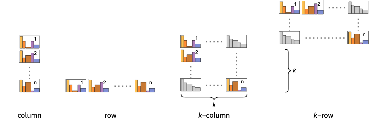
-
"Column" use separate charts in a column of panels "Row" use separate charts in a row of panels {"Column",k},{"Row",k} use k columns or rows {"Column",UpTo[k]},{"Row",UpTo[k]} use at most k columns or rows - Typical settings for PlotLegends include:
-
None no legend Automatic automatically determine legend {lbl1,lbl2,…} use lbl1, lbl2, … as legend labels Placed[lspec,…] specify placement for legend - PlotStylesty specifies the styles to use for each curve. Possible settings include:
-
{sty1,sty2,…} sequence of styles for the data <"key"val,…> styling elements for different levels of data - The accepted keys are:
-
"Base" overall style for all the bars "Elements" list of styles for the elements yi in each group "Groups" list of styles of each group of values datai - ColorData["DefaultChartColors"] gives the default sequence of colors used by PlotStyle.
- The arguments supplied to ChartElementFunction are the bar region {{xmin,xmax},{ymin,ymax}}, the data value {xi,yi}, and metadata {m1,m2,…} from each level in a nested list of datasets.
- A list of built-in settings for ChartElementFunction can be obtained from ChartElementData["RectangleChart"].
- The arguments supplied to ColorFunction consist of xi and yi.
- Style and other specifications from options and other constructs in RectangleChart are effectively applied in the order PlotStyle, ColorFunction, Style and other wrappers, ChartElements, and ChartElementFunction, with later specifications overriding earlier ones.
List of all options
Examples
open all close allBasic Examples (4)
Generate a rectangle chart for a list of width and height pairs:
RectangleChart[{{1, 1}, {1, 2}, {2, 3}}]RectangleChart[{{{1, 1}, {1, 2}, {2, 3}}, {{3, 2}, {1, 3}, {2, 1}}}]Show multiple sets as a row of charts:
RectangleChart[{{{1, 1}, {1, 2}, {2, 3}}, {{3, 2}, {1, 3}, {2, 1}}}, ChartLayout -> "Row"]data = {{{1, 1}, {1, 2}, {2, 3}}, {{1, 1}, {2, 1}}};RectangleChart[data, PlotLabels -> <|"Elements" -> {"a", "b", "c"}|>]RectangleChart[data, PlotLegends -> <|"Elements" -> {"a", "b", "c"}|>]RectangleChart[Tuples[{1, 2}, 2], PlotStyle -> {RGBColor[0.237736, 0.340215, 0.575113], RGBColor[0.33311066666666667, 0.5032283333333333, 0.26154733333333335], RGBColor[0.8562609999999999, 0.742794, 0.31908333333333333], RGBColor[0.72987, 0.239399, 0.230961]}]RectangleChart[Tuples[{1, 2}, 2], ChartElements -> {[image], {All, 1}}]RectangleChart[Tuples[{1, 2}, 2], ChartElementFunction -> "GlassRectangle", PlotStyle -> {RGBColor[0.761959, 0.470832, 0.940597], RGBColor[0.927848, 0.742785, 0.6151383333333333], RGBColor[0.929162, 0.95034, 0.6648153333333333], RGBColor[0.431296, 0.709773, 0.927077]}]Scope (41)
Data and Layouts (13)
Items in a dataset are grouped together:
RectangleChart[{{{1, 1}, {1, 1}, {1, 1}}, {{2, 2}, {2, 2}, {2, 2}}}]Datasets do not need to have the same number of items:
RectangleChart[{{{1, 1}, {1, 2}, {2, 3}}, {{1, 1}, {2, 1}}}]Non-real data is taken to be missing:
RectangleChart[{{{1, 1}, Missing[], {1, 1}, {1, 1}}, {{2, 2}, 1 + I, {2, 2}}, {foo, {3, 3}}}]RectangleChart[{{Quantity[3, "Seconds"], Quantity[2, "Meters"]}, {Quantity[8, "Seconds"], Quantity[5, "Meters"]}, {Quantity[2, "Seconds"], Quantity[3, "Meters"]}, {Quantity[1, "Seconds"], Quantity[3, "Meters"]}, {Quantity[8, "Seconds"], Quantity[7, "Meters"]}, {Quantity[7, "Seconds"], Quantity[1, "Meters"]}}, AxesLabel -> Automatic, BarSpacing -> None, Ticks -> True]RectangleChart[{{Quantity[3, "Seconds"], Quantity[2, "Meters"]}, {Quantity[8, "Seconds"], Quantity[5, "Meters"]}, {Quantity[2, "Seconds"], Quantity[3, "Meters"]}, {Quantity[1, "Seconds"], Quantity[3, "Meters"]}, {Quantity[8, "Seconds"], Quantity[7, "Meters"]}, {Quantity[7, "Seconds"], Quantity[1, "Meters"]}}, AxesLabel -> Automatic, BarSpacing -> None, Ticks -> True, TargetUnits -> {"Minutes", "Feet"}]The time stamps in TimeSeries, EventSeries, and TemporalData are ignored:
RectangleChart[TimeSeries[{{19, 16}, {9, 3}, {7, 2}, {17, 5}}, {"May 24, 1982"}]]The values in associations are taken as the dimensions of the bars:
RectangleChart[<|"a" -> {1, 1}, "b" -> {1, 2}, "c" -> {2, 1}, "d" -> {2, 2}|>]RectangleChart[<|"a" -> {1, 1}, "b" -> {1, 2}, "c" -> {2, 1}, "d" -> {2, 2}|>, PlotLabels -> Automatic]RectangleChart[<|"a" -> {1, 1}, "b" -> {1, 2}, "c" -> {2, 1}, "d" -> {2, 2}|>, PlotLabels -> Callout[Automatic, Above]]RectangleChart[<|"a" -> {1, 1}, "b" -> {1, 2}, "c" -> {2, 1}, "d" -> {2, 2}|>, PlotLegends -> Automatic, PlotStyle -> {RGBColor[0.65, 0., 0.], RGBColor[0.0504678, 0.526626, 0.627561], RGBColor[0.752461, 0.362306, 0.125339], RGBColor[0.435888, 0.259065, 0.71028]}]RectangleChart[<|"group a" -> <|"a" -> {1, 2}, "b" -> {2, 1}|>, "group b" -> <|"a" -> {1, 1}, "b" -> {2, 2}|>|>, PlotLegends -> Automatic]The weights in WeightedData are ignored:
RectangleChart[WeightedData[{{1, 1}, {2, 1}, {3, 2}, {4, 3}, {5, 5}}, {0.5, 0.2, 0.1, 0.2, 0.3}]]Use different layouts to display multiple datasets:
Table[RectangleChart[Tuples[{1, 2}, 2], ChartLayout -> l], {l, {"Grouped", "Stepped"}}]RectangleChart[{IconizedObject[«data #1»], IconizedObject[«data #2»], IconizedObject[«data #3»]}, ImageSize -> Medium, ChartLayout -> "Row"]Use a column of sector charts:
RectangleChart[{IconizedObject[«data #1»], IconizedObject[«data #2»], IconizedObject[«data #3»]}, ImageSize -> Medium, ChartLayout -> "Column"]RectangleChart[{IconizedObject[«data #1»], IconizedObject[«data #2»], IconizedObject[«data #3»], IconizedObject[«data #4»]}, ImageSize -> Medium, ChartLayout -> {"Row", 2}]Table[RectangleChart[{{1, 1}, {1, 2}, {2, 3}}, BarOrigin -> o, PlotLabel -> o], {o, {Bottom, Left, Top, Right}}]Adjust the spacing between bars and groups of bars:
Table[RectangleChart[Tuples[{1, 2}, 2], BarSpacing -> s, PlotLabel -> s, PlotStyle -> Opacity[0.8]], {s, {Automatic, {0, 1}, {-0.3, 1}}}]Tabular Data (3)
tabdata = AggregateRows[Tabular[ResourceData["Sample Data: 1993 US Cars"]], {"AvgPrice" -> (Mean[#AvgPrice]&), "TotalCars" -> (Length[#AvgPrice]&), "AvgWeight" -> (Mean[#Weight]&), "AvgFuelTankCap" -> (Mean[#FuelTankCapacity]&)}, {"Type"}]Compare the average price of each group of cars along the number of cars:
RectangleChart[tabdata -> {"TotalCars", "AvgPrice"}, PlotLabels -> Normal[tabdata[All, "Type"]]]Plot the values for all the components in TimeSeries or EventSeries:
RectangleChart[TimeSeries[TimeEventSeries`TimestampData[Association["UniformlySpacedQ" -> True, "Count" -> 5,
   "Endpoints" -> TabularColumn[Association[
      "Data" -> {2, {{NumericArray[{20563, -2147483648}, "Integer32"], {},
          DataStructure["BitVec ...   {{TabularColumn[Association["Data" -> {{1, 1, 2, 5, 8}, {}, None},
           "ElementType" -> "Integer64"]], TabularColumn[Association[
           "Data" -> {{2, 2, 16, 17, 17}, {}, None}, "ElementType" -> "Integer64"]]}}]]]],
 Association[]]]
Plot the values for a set of components of a TimeSeries or EventSeries:
ts = TimeSeries[TimeEventSeries`TimestampData[Association["UniformlySpacedQ" -> True, "Count" -> 5,
   "Endpoints" -> TabularColumn[Association[
      "Data" -> {2, {{NumericArray[{20563, -2147483648}, "Integer32"], {},
          DataStructure["BitVec ... larColumn[Association[
           "Data" -> {{2, 2, 16, 17, 17}, {}, None}, "ElementType" -> "Integer64"]],
         TabularColumn[Association["Data" -> {{5, 5, 4, 4, 2}, {}, None},
"ElementType" -> "Integer64"]]}}]]]], Association[]];RectangleChart[ts -> {"a", "b"}]Plot values from multiple sets of components:
RectangleChart[ts -> {{"a", "b"}, {"a", "c"}}]Wrappers (5)
Use wrappers on individual data, datasets, or collections of datasets:
{RectangleChart[{{{1, 1}, Style[{1, 2}, RGBColor[0.93, 0.27, 0.27]], {2, 3}}, {{1, 1}, {2, 1}}}], RectangleChart[{Style[{{1, 1}, {1, 2}, {2, 3}}, RGBColor[0.14, 0.8, 0.14]], {{1, 1}, {2, 1}}}], RectangleChart[Style[{{{1, 1}, {1, 2}, {2, 3}}, {{1, 1}, {2, 1}}}, RGBColor[0.4, 0.6, 1]]]}{RectangleChart[{{{1, 1}, Style[{1, 2}, RGBColor[0.93, 0.27, 0.27]], {2, 3}}, {{1, 1}, {2, 1}}}], RectangleChart[{Style[{{1, 1}, Style[{1, 2}, RGBColor[0.93, 0.27, 0.27]], {2, 3}}, RGBColor[0.14, 0.8, 0.14]], {{1, 1}, {2, 1}}}], RectangleChart[Style[{Style[{{1, 1}, Style[{1, 2}, RGBColor[0.93, 0.27, 0.27]], {2, 3}}, RGBColor[0.14, 0.8, 0.14]], {{1, 1}, {2, 1}}}, RGBColor[0.4, 0.6, 1]]]}Override the default tooltips:
RectangleChart[{{1, 1}, Tooltip[{1, 2}, "median"], {2, 3}}]Use any object in the tooltip:
RectangleChart[Table[Tooltip[{CountryData[c, "Population"], CountryData[c, "GDPPerCapita"]}, CountryData[c, "Flag"]], {c, CountryData["G8"]}], BarSpacing -> 0]Use PopupWindow to provide additional drilldown information:
RectangleChart[{{1, 1}, PopupWindow[{1, 2}, DateListPlot[FinancialData["IBM", "Jan. 1, 2004"]]], {2, 3}}]Button can be used to trigger any action:
RectangleChart[{{1, 1}, Button[{1, 2}, Speak[2]], {2, 3}}]Styling and Appearance (7)
Use an explicit list of styles for the bars:
RectangleChart[{{1, 1}, {1, 2}, {2, 3}}, PlotStyle -> {RGBColor[0.93, 0.27, 0.27], RGBColor[0.14, 0.8, 0.14], RGBColor[0.4, 0.6, 1]}]Alter the appearance of charts with built-in themes:
{RectangleChart[{{1, 1}, {1, 2}, {2, 3}}, PlotTheme -> "Marketing"], RectangleChart[{{1, 1}, {1, 2}, {2, 3}}, PlotTheme -> "Detailed"]}PlotStyle can be used to set an initial style for all chart elements:
RectangleChart[{{1, 1}, {1, 2}, {2, 3}}, PlotStyle -> <|"Base" -> EdgeForm[Dashed], "Elements" -> {RGBColor[0.797253, 0.904982, 0.410498], RGBColor[0.934691, 0.945708, 0.75346], RGBColor[0.769879, 0.92369, 0.977371]}|>]Style can be used to override styles:
RectangleChart[{{1, 1}, {1, 2}, Style[{3, 4}, RGBColor[0.93, 0.27, 0.27]], {2, 3}}, PlotStyle -> GrayLevel[0.62]]Use any graphic for pictorial bars:
{RectangleChart[{{1, 1}, {1, 2}, {2, 3}}, ChartElements -> Graphics[Disk[]]], RectangleChart[{{1, 1}, {1, 2}, {2, 3}}, ChartElements -> ExampleData[{"TestImage", "House"}]]}Use built-in programmatically generated bars:
ChartElementData["RectangleChart"]Table[RectangleChart[{{1, 1}, {1, 2}, {2, 3}}, ChartElementFunction -> f, PlotStyle -> {RGBColor[0.761959, 0.470832, 0.940597], RGBColor[0.9584254999999999, 0.877884, 0.5906629999999999], RGBColor[0.431296, 0.709773, 0.927077]}], {f, {"FadingRectangle", "GlassRectangle"}}]For detailed settings use Palettes ▶ ChartElementSchemes:
RectangleChart[{{1, 1}, {1, 2}, {2, 3}}, ChartElementFunction -> ChartElementDataFunction["SegmentScaleRectangle", "Segments" -> 7, "ColorScheme" -> "SolarColors"]]Use a theme with detailed frame ticks and grid lines:
RectangleChart[{{{1, 1}, {1, 2}, {2, 3}}, {{2, 1}, {1, 2}}}, PlotTheme -> "Detailed"]Use a theme with a high-contrast color scheme and edge-fading rectangles:
RectangleChart[{{{1, 1}, {1, 2}, {2, 3}}, {{2, 1}, {1, 2}}}, PlotTheme -> "Marketing"]Labeling and Legending (13)
Use Labeled to add a label to a bar:
RectangleChart[{{1, 1}, Labeled[{1, 2}, "label"], {2, 3}}]Use symbolic positions for label placement:
Table[RectangleChart[{{1, 1}, Labeled[{1, 2}, "label", p], {2, 3}}, PlotLabel -> p, Ticks -> None], {p, {Bottom, Center, Top}}]Table[RectangleChart[{{1, 1}, Labeled[{1, 2}, "label", p], {2, 3}}, BarOrigin -> Left, PlotLabel -> p, Ticks -> None], {p, {Left, Center, Right}}]Specify categorical labels for data elements:
RectangleChart[{{{1, 1}, {1, 2}, {2, 3}}, {{1, 1}, {2, 1}}}, PlotLabels -> <|"Elements" -> {"c1", "c2", "c3"}|>]RectangleChart[{{{1, 1}, {1, 2}, {2, 3}}, {{1, 1}, {2, 1}}}, PlotLabels -> <|"Groups" -> {"r1", "r2"}|>]RectangleChart[{{{1, 1}, {1, 2}, {2, 3}}, {{1, 1}, {2, 1}}}, PlotLabels -> <|"Elements" -> {"c1", "c2", "c3"}, "Groups" -> {"r1", "r2"}|>]Use Placed to control the positioning of labels, using the same positions as for Labeled:
RectangleChart[{{{1, 1}, {1, 2}, {2, 3}}, {{1, 1}, {2, 1}}}, PlotLabels -> <|"Elements" -> Placed[{"c1", "c2", "c3"}, Center], "Groups" -> Placed[{"r1", "r2"}, Above]|>]Use Callout to add a label to a bar:
RectangleChart[{{1, 1}, {1, 2}, Callout[{2, 3}, "label"]}]Change the appearance of the callout:
RectangleChart[{{1, 1}, {1, 2}, Callout[{2, 3}, "label", Appearance -> "Balloon"]}]Automatically position callouts:
RectangleChart[Table[Callout[RandomReal[{1, 5}, 2], Unique["text"]], 5]]Provide value labels for bars by using LabelingFunction:
RectangleChart[{{1, 1}, {1, 2}, {2, 3}}, LabelingFunction -> Above]Use Placed to control placement and formatting:
labeler[v_, {i_, j_}, {ri_, cj_}] := Placed[Column[{v, ri[[1]], cj[[1]]}, ","], Center]RectangleChart[{{{1, 1}, {1, 2}, {2, 3}}, {{1, 1}, {2, 1}}}, PlotLabels -> <|"Groups" -> {"r1", "r2"}, "Elements" -> {"c1", "c2", "c3"}|>, LabelingFunction -> labeler]Generate callouts from the data:
RectangleChart[{{1, 4}, {5, 5}, {1, 1}, {4, 1}, {2, 3}}, LabelingFunction -> (Callout[Style[Times@@#, 10 + 5Max[#]], Above]&)]Add categorical legend entries for data elements:
RectangleChart[{{{1, 1}, {1, 2}, {2, 3}}, {{1, 1}, {2, 1}}}, PlotLegends -> <|"Elements" -> {"ccc1", "ccc2", "ccc3"}|>, PlotStyle -> <|"Elements" -> {RGBColor[0.761959, 0.470832, 0.940597], RGBColor[0.9584254999999999, 0.877884, 0.5906629999999999], RGBColor[0.431296, 0.709773, 0.927077]}|>]RectangleChart[{{{1, 1}, {1, 2}, {2, 3}}, {{1, 1}, {2, 1}}}, PlotLegends -> {"rr1", "rr2"}, PlotStyle -> <|"Groups" -> "Pastel"|>]Use Legended to add additional legend entries:
RectangleChart[{{{1, 1}, Legended[{1, 2}, "extra"], {2, 3}}, {{1, 1}, {2, 1}}}, PlotStyle -> <|"Elements" -> {RGBColor[0.761959, 0.470832, 0.940597], RGBColor[0.9584254999999999, 0.877884, 0.5906629999999999], RGBColor[0.431296, 0.709773, 0.927077]}|>, PlotLegends -> <|"Elements" -> {"aaa", "bbb", "ccc"}|>]Use Placed to affect the positioning of legends:
Table[RectangleChart[{{{1, 1}, {1, 2}, {2, 3}}, {{1, 1}, {2, 1}}}, PlotLegends -> <|"Elements" -> Placed[{"ccc1", "ccc2", "ccc3"}, p]|>, PlotStyle -> <|"Elements" -> {RGBColor[0.761959, 0.470832, 0.940597], RGBColor[0.9584254999999999, 0.877884, 0.5906629999999999], RGBColor[0.431296, 0.709773, 0.927077]}|>], {p, {Before, Below}}]Options (95)
AspectRatio (4)
By default, RectangleChart uses a fixed height-to-width ratio for the plot:
RectangleChart[{{1, 1}, {1, 2}, {2, 3}, {3, 1}, {1, 4}, {2, 2}}]Make the height the same as the width with AspectRatio1:
RectangleChart[{{1, 1}, {1, 2}, {2, 3}, {3, 1}, {1, 4}, {2, 2}}, AspectRatio -> 1]AspectRatioAutomatic determines the ratio from the data:
RectangleChart[{{1, 1}, {1, 2}, {2, 3}, {3, 1}, {1, 4}, {2, 2}}, AspectRatio -> Automatic]AspectRatioFull adjusts the height and width to fit tightly inside other constructs:
plot = RectangleChart[{{1, 1}, {1, 2}, {2, 3}, {3, 1}, {1, 4}, {2, 2}}, AspectRatio -> Full];{Framed[Pane[plot, {50, 100}]], Framed[Pane[plot, {100, 100}]], Framed[Pane[plot, {100, 50}]]}Axes (3)
RectangleChart[{{1, 1}, {1, 2}, {2, 3}, {3, 1}, {1, 4}, {2, 2}}]Use AxesFalse to turn off axes:
RectangleChart[{{1, 1}, {1, 2}, {2, 3}, {3, 1}, {1, 4}, {2, 2}}, Axes -> False]Turn each axis on individually:
{RectangleChart[{{1, 1}, {1, 2}, {2, 3}, {3, 1}, {1, 4}, {2, 2}}, Axes -> {False, True}], RectangleChart[{{1, 1}, {1, 2}, {2, 3}, {3, 1}, {1, 4}, {2, 2}}, Axes -> {True, False}]}AxesStyle (4)
Change the style for the axes:
RectangleChart[{{1, 1}, {1, 2}, {2, 3}, {3, 1}, {1, 4}, {2, 2}}, AxesStyle -> RGBColor[0.93, 0.27, 0.27]]Specify the style of each axis:
RectangleChart[{{1, 1}, {1, 2}, {2, 3}, {3, 1}, {1, 4}, {2, 2}}, AxesStyle -> {RGBColor[0.93, 0.27, 0.27], RGBColor[0.4, 0.6, 1]}]Use different styles for the ticks and the axes:
RectangleChart[{{1, 1}, {1, 2}, {2, 3}, {3, 1}, {1, 4}, {2, 2}}, AxesStyle -> RGBColor[0.14, 0.8, 0.14], TicksStyle -> RGBColor[0.4, 0.6, 1]]Use different styles for the labels and the axes:
RectangleChart[{{1, 1}, {1, 2}, {2, 3}, {3, 1}, {1, 4}, {2, 2}}, AxesStyle -> RGBColor[0.14, 0.8, 0.14], LabelStyle -> RGBColor[0.4, 0.6, 1]]BarOrigin (1)
BarSpacing (5)
Use automatically determined spacing between bars:
RectangleChart[{{{1, 1}, {1, 2}, {2, 3}}, {{1, 1}, {2, 1}}}, BarSpacing -> Automatic]RectangleChart[{{{1, 1}, {1, 2}, {2, 3}}, {{1, 1}, {2, 1}}}, BarSpacing -> None]Table[RectangleChart[{{{1, 1}, {1, 2}, {2, 3}}, {{1, 1}, {2, 1}}}, BarSpacing -> s, PlotLabel -> s], {s, {Tiny, Small, Medium, Large}}]Use explicit spacing between bars:
Table[RectangleChart[{{{1, 1}, {1, 2}, {2, 3}}, {{1, 1}, {2, 1}}}, BarSpacing -> s, PlotStyle -> Opacity[0.8], PlotLabel -> s], {s, {Automatic, 1, -0.3}}]Use explicit spacing between bars and groups of bars:
Table[RectangleChart[{{{1, 1}, {1, 2}, {2, 3}}, {{1, 1}, {2, 1}}}, BarSpacing -> s, PlotLabel -> s], {s, {Automatic, {0, 1}, {0, 0.2}}}]ChartElementFunction (5)
Get a list of built-in settings for ChartElementFunction:
ChartElementData["RectangleChart"]For detailed settings use Palettes ▶ ChartElementSchemes:
Table[RectangleChart[Tuples[{1, 2}, 2], ChartElementFunction -> f, PlotStyle -> {RGBColor[0.761959, 0.470832, 0.940597], RGBColor[0.927848, 0.742785, 0.6151383333333333], RGBColor[0.929162, 0.95034, 0.6648153333333333], RGBColor[0.431296, 0.709773, 0.927077]}, PlotLabel -> f], {f, {"Rectangle", "ObliqueRectangle"}}]Table[RectangleChart[Tuples[{1, 2}, 2], ChartElementFunction -> f, PlotStyle -> {RGBColor[0.761959, 0.470832, 0.940597], RGBColor[0.927848, 0.742785, 0.6151383333333333], RGBColor[0.929162, 0.95034, 0.6648153333333333], RGBColor[0.431296, 0.709773, 0.927077]}, PlotLabel -> f], {f, {"FadingRectangle", "GlassRectangle"}}]Here is a ChartElementFunction appropriate to show the global scale:
Table[RectangleChart[Tuples[{1, 2}, 2], ChartElementFunction -> f, PlotStyle -> {RGBColor[0.761959, 0.470832, 0.940597], RGBColor[0.927848, 0.742785, 0.6151383333333333], RGBColor[0.929162, 0.95034, 0.6648153333333333], RGBColor[0.431296, 0.709773, 0.927077]}, PlotLabel -> f], {f, {"GradientScaleRectangle", "SegmentScaleRectangle"}}]Write a custom ChartElementFunction:
f[{{xmin_, xmax_}, {ymin_, ymax_}}, ___] := Rectangle[{xmin, ymin}, {xmax, ymax}]RectangleChart[Tuples[{1, 2}, 2], ChartElementFunction -> f]g[{{xmin_, xmax_}, {ymin_, ymax_}}, ___] := Polygon[{{xmin, ymin}, {xmax, ymax}, {xmin, ymax}, {xmax, ymin}}]RectangleChart[Tuples[{1, 2}, 2], ChartElementFunction -> g]Use metadata passed on from the input, in this case charting the data:
DataDrilldownBar[{{xmin_, xmax_}, {ymin_, ymax_}}, y_, {data_List}] :=
PopupWindow[Polygon[{{xmin, ymin}, {xmax, ymax}, {xmin, ymax}, {xmax, ymin}}], PieChart[data]]DataDrilldownBar[{{xmin_, xmax_}, {ymin_, ymax_}}, y_, _] :=
Rectangle[{xmin, ymin}, {xmax, ymax}]RectangleChart[{{1, 1} -> Range[5], {1, 2}, {2, 1} -> RandomReal[1, 10]}, ChartElementFunction -> DataDrilldownBar]ChartElements (9)
Create a pictorial chart based on any Graphics object:
RectangleChart[Tuples[{1, 2}, 2], ChartElements -> Graphics[Disk[]]]RectangleChart[Tuples[{1, 2}, 2], ChartElements -> Graphics3D[Sphere[]]]RectangleChart[Tuples[{1, 2}, 2], ChartElements -> ExampleData[{"TestImage", "House"}]]Use a stretched version of the graphic:
RectangleChart[Tuples[{1, 2}, 2], ChartElements -> {[image], All}]Use explicit sizes for width and height:
Table[RectangleChart[Tuples[{1, 2}, 2], ChartElements -> {Graphics[Disk[], AspectRatio -> Full], s}, PlotLabel -> s], {s, {{1 / 2, 1}, {1, 1 / 2}}}]Without AspectRatio->Full, the original aspect ratio is preserved:
Table[RectangleChart[Tuples[{1, 2}, 2], ChartElements -> {Graphics[Disk[]], s}, PlotLabel -> s], {s, {{1 / 2, 1}, {1, 1 / 2}}}]Using All for width or height causes that direction to stretch to the full size of the bar:
Table[RectangleChart[Tuples[{1, 2}, 2], ChartElements -> {[image], s}, PlotLabel -> s], {s, {{1 / 2, All}, {All, 1 / 2}}}]Use a different graphic for each column of data:
RectangleChart[{{{1, 1}, {1, 2}, {2, 3}}, {{1, 1}, {2, 1}}}, ChartElements -> {[image], [image], [image]}]Use a different graphic for each row of data:
RectangleChart[{{{1, 1}, {1, 2}, {2, 3}}, {{1, 1}, {2, 1}}}, ChartElements -> {{[image], [image]}, None}]RectangleChart[Tuples[{1, 2}, 2], ChartElements -> {{[image], All}, {[image], All}}]Styles are inherited from styles set through PlotStyle etc.:
RectangleChart[Tuples[{1, 2}, 2], ChartElements -> [image], PlotStyle -> {RGBColor[0.761959, 0.470832, 0.940597], RGBColor[0.927848, 0.742785, 0.6151383333333333], RGBColor[0.929162, 0.95034, 0.6648153333333333], RGBColor[0.431296, 0.709773, 0.927077]}]Explicit styles set in the graphic will override other style settings:
RectangleChart[Tuples[{1, 2}, 2], ChartElements -> [image], PlotStyle -> {RGBColor[0.761959, 0.470832, 0.940597], RGBColor[0.927848, 0.742785, 0.6151383333333333], RGBColor[0.929162, 0.95034, 0.6648153333333333], RGBColor[0.431296, 0.709773, 0.927077]}]The orientation of the pictorial graphic is unaffected by BarOrigin:
Table[RectangleChart[Tuples[{1, 2}, 2], ChartElements -> [image], BarOrigin -> o], {o, {Bottom, Top, Left, Right}}]g = Graphics3D[{EdgeForm[], Specularity[White, 30], Cylinder[]}, ViewPoint -> {0, -Infinity, 0}, Boxed -> False, Lighting -> "Neutral", PlotRangePadding -> 0];RectangleChart[Tuples[{1, 2}, 2], ChartElements -> {g, All}]ColorFunction (4)
RectangleChart[Table[{Exp[-t ^ 2], Exp[-t ^ 2]}, {t, -2, 2, 0.25}], ColorFunction -> Function[{width, height}, ColorData["Rainbow"][height]]]Use ColorFunctionScaling->False to get unscaled height values:
RectangleChart[Tuples[{1, 2}, 2], ColorFunction -> (Switch[{#1, #2}, {1, 1}, RGBColor[1, 0.75, 0], {1, 2}, RGBColor[0.98, 0.56, 0.17], {2, 1}, RGBColor[0.93, 0.27, 0.27], _, RGBColor[0.4, 0.6, 1]]&), ColorFunctionScaling -> False]RectangleChart[{{1, 1}, {1, 2}, {2, 1}, {2, 2}}, ColorFunction -> Function[{width, height}, ColorData["Rainbow"][width height / 4]], ColorFunctionScaling -> False]ColorFunction overrides styles in PlotStyle:
ColorData["Pastel"] /@ Range[0, 1, 1 / 2]RectangleChart[Tuples[{1, 2, 3}, 2], PlotStyle -> {RGBColor[0.93, 0.27, 0.27], RGBColor[0.14, 0.8, 0.14], RGBColor[0.67, 0.54, 0.42]}, ColorFunction -> {RGBColor[0.761959, 0.470832, 0.940597], RGBColor[0.9584254999999999, 0.877884, 0.5906629999999999], RGBColor[0.431296, 0.709773, 0.927077]}]Use ColorFunction to combine different style effects:
RectangleChart[Table[{Exp[-t ^ 2], Exp[-t ^ 2]}, {t, -2, 2, 0.25}], ColorFunction -> Function[{width, height}, Opacity[height]], PlotStyle -> RGBColor[0.8, 0.3, 0.8]]ColorFunctionScaling (2)
Use ColorFunctionScaling->False to get unscaled height values:
RectangleChart[Tuples[{1, 2}, 2], ColorFunction -> (Switch[{#1, #2}, {1, 1}, RGBColor[1, 0.75, 0], {1, 2}, RGBColor[0.98, 0.56, 0.17], {2, 1}, RGBColor[0.93, 0.27, 0.27], _, RGBColor[0.4, 0.6, 1]]&), ColorFunctionScaling -> False]RectangleChart[{{1, 1}, {1, 2}, {2, 1}, {2, 2}}, ColorFunction -> Function[{width, height}, ColorData["Rainbow"][width height / 4]], ColorFunctionScaling -> False]ImageSize (7)
Use named sizes, such as Tiny, Small, Medium and Large:
{RectangleChart[IconizedObject[«data»], ImageSize -> Tiny], RectangleChart[IconizedObject[«data»], ImageSize -> Small]}Specify the width of the plot:
{RectangleChart[IconizedObject[«data»], ImageSize -> 150], RectangleChart[IconizedObject[«data»], AspectRatio -> 1.5, ImageSize -> 150]}Specify the height of the plot:
{RectangleChart[IconizedObject[«data»], ImageSize -> {Automatic, 150}], RectangleChart[IconizedObject[«data»], AspectRatio -> 2, ImageSize -> {Automatic, 150}]}Allow the width and height to be up to a certain size:
{RectangleChart[IconizedObject[«data»], ImageSize -> UpTo[200]], RectangleChart[IconizedObject[«data»], AspectRatio -> 2, ImageSize -> UpTo[200]]}Specify the width and height for a graphic, padding with space if necessary:
RectangleChart[IconizedObject[«data»], ImageSize -> {200, 200}, Background -> GrayLevel[0.62]]Setting AspectRatioFull will fill the available space:
RectangleChart[IconizedObject[«data»], AspectRatio -> Full, ImageSize -> {200, 200}, Background -> GrayLevel[0.62]]Use maximum sizes for the width and height:
{RectangleChart[IconizedObject[«data»], ImageSize -> {UpTo[150], UpTo[100]}], RectangleChart[IconizedObject[«data»], AspectRatio -> 2, ImageSize -> {UpTo[150], UpTo[100]}]}Use ImageSizeFull to fill the available space in an object:
Framed[Pane[RectangleChart[IconizedObject[«data»], ImageSize -> Full, Background -> GrayLevel[0.62]], {200, 100}]]Specify the image size as a fraction of the available space:
Framed[Pane[RectangleChart[IconizedObject[«data»], AspectRatio -> Full, ImageSize -> {Scaled[0.5], Scaled[0.5]}, Background -> GrayLevel[0.62]], {200, 100}]]LabelingFunction (8)
Use automatic labeling by values through Tooltip and StatusArea:
RectangleChart[{{1, 1}, {1, 2}, {2, 3}}, LabelingFunction -> Automatic]RectangleChart[{{1, 1}, {1, 2}, {2, 3}}, LabelingFunction -> None]Use Placed to control label placement:
Table[RectangleChart[{{1, 1}, {1, 2}, {2, 3}}, LabelingFunction -> (Placed[#, p]&), PlotLabel -> p, Ticks -> None], {p, {Bottom, Center, Top}}]Symbolic positions outside the bar:
Table[RectangleChart[{{1, 1}, {1, 2}, {2, 3}}, LabelingFunction -> (Placed[#, p]&), PlotLabel -> p, Ticks -> None], {p, {Below, Above}}]Table[RectangleChart[{{1, 1}, {1, 2}, {2, 3}}, LabelingFunction -> (Placed[#, p]&), BarOrigin -> Left, PlotLabel -> p, Ticks -> None], {p, {Before, After}}]Coordinate-based placement relative to a bar:
Table[RectangleChart[{{1, 1}, {1, 2}, {2, 3}}, LabelingFunction -> (Placed[#, p]&), BarSpacing -> 0.5, Ticks -> None, PlotLabel -> p], {p, {{0, 0}, {1 / 2, 1 / 2}, {1, 1}}}]Use Callout to place labels automatically:
RectangleChart[{{3, 5}, {8, 4}, {6, 7}}, LabelingFunction -> (Callout[Row[#, "⊗"], Automatic]&)]Use symbolic positions to place Callout labels:
Table[RectangleChart[{{3, 5}, {8, 4}, {6, 7}}, LabelingFunction -> (Callout[#, p]&)], {p, {Above, Below}}]Control the formatting of labels:
RectangleChart[{{1, 1}, {1, 2}, {2, 3}}, LabelingFunction -> (Placed[Row[#, "to"], Above]&)]Use the given chart labels as arguments to the labeling function:
data = {{{1, 1}, {1, 2}, {2, 3}}, {{1, 1}, {2, 1}}};RectangleChart[data, PlotLabels -> <|"Groups" -> {"r1", "r2"}, "Elements" -> {"c1", "c2", "c3"}|>, LabelingFunction -> (Placed[Column[{#3[[1, 1]], #3[[2, 1]], #1}, ","], Center]&), ImageSize -> Medium]Place complete labels as tooltips:
RectangleChart[data, PlotLabels -> <|"Groups" -> {"r1", "r2"}, "Elements" -> {"c1", "c2", "c3"}|>, LabelingFunction -> (Placed[Row[{#3[[1, 1]], #3[[2, 1]], #1}, ","], Tooltip]&)]LabelingSize (4)
Textual labels are shown at their actual sizes:
RectangleChart[{{1, 1}, {1, 2}, {2, 3}, {3, 2}}, PlotLabels -> {"healthfulness", "obstreperous", "spectrogram", "pandemonium"}]Image labels are automatically resized:
RectangleChart[{{1, 1}, {1, 2}, {2, 3}, {3, 2}}, PlotLabels -> {[image], [image], [image], [image]}]Specify a maximum size for textual labels:
RectangleChart[{{1, 1}, {1, 2}, {2, 3}, {3, 2}}, PlotLabels -> {"healthfulness", "obstreperous", "spectrogram", "pandemonium"}, LabelingSize -> 50]Specify a maximum size for image labels:
RectangleChart[{{1, 1}, {1, 2}, {2, 3}, {3, 2}}, PlotLabels -> {[image], [image], [image], [image]}, LabelingSize -> 25]Show image labels at their natural sizes:
RectangleChart[{{1, 1}, {1, 2}, {2, 3}, {3, 2}}, PlotLabels -> Placed[{[image], [image], [image], [image]}, Above], LabelingSize -> Full, ImageSize -> Medium]PerformanceGoal (3)
Generate a bar chart with interactive highlighting:
RectangleChart[Tuples[{1, 2, 3}, 2], PerformanceGoal -> "Quality"]Emphasize performance by disabling interactive behaviors:
RectangleChart[Tuples[{1, 2, 3}, 2], PerformanceGoal -> "Speed"]Typically, less memory is required for non-interactive charts:
Table[ByteCount@RectangleChart[Tuples[{1, 2, 3}, 2], PerformanceGoal -> p], {p, {"Quality", "Speed"}}]PlotInteractivity (4)
Charts with a moderate number of bars automatically have tooltips and mouseover effects:
RectangleChart[{{1, 1}, {2, 2}, {2, 1}}]Turn off all the interactive elements:
RectangleChart[{{1, 1}, {2, 2}, {2, 1}}, PlotInteractivity -> False]Interactive elements provided as part of the input are disabled:
RectangleChart[{{1, 1}, {2, 2}, Tooltip[{2, 1}, "Hello"]}, PlotInteractivity -> False]Allow provided interactive elements and disable automatic ones:
RectangleChart[{{1, 1}, {2, 2}, Tooltip[{2, 1}, "Hello"]}, PlotInteractivity -> <|"User" -> True, "System" -> False|>]PlotLabels (9)
By default, labels are placed in the axis:
RectangleChart[{{1, 1}, {1, 2}, {2, 3}}, PlotLabels -> {"a", "b", "c"}]RectangleChart[{{{1, 1}, {1, 2}, {2, 3}}, {{1, 1}, {2, 1}}}, PlotLabels -> {"a", "b"}]By default, labels are associated with data elements or groups automatically:
{RectangleChart[{{1, 1}, {1, 2}, {2, 3}}, PlotLabels -> {"c1", "c2", "c3"}],
	RectangleChart[{{{1, 1}, {1, 2}, {2, 3}}, {{1, 1}, {2, 1}}}, PlotLabels -> {"r1", "r2", "r3"}]}
Specify labels to data elements specifically:
RectangleChart[{{{1, 1}, {1, 2}, {2, 3}}, {{1, 1}, {2, 1}}}, PlotLabels -> <|"Elements" -> {"c1", "c2", "c3"}|>]Label both groups and elements:
RectangleChart[{{{1, 1}, {1, 2}, {2, 3}}, {{1, 1}, {2, 1}}}, PlotLabels -> <|"Groups" -> {"r1", "r2"}, "Elements" -> {"c1", "c2", "c3"}|>]Labeled wrappers in data will place additional labels:
RectangleChart[{{1, 1}, Labeled[{1, 2}, "label", Center], {2, 3}}, PlotLabels -> {"a", "b", "c"}]Use Placed to control label placement:
Table[RectangleChart[{{1, 1}, {1, 2}, {2, 3}}, PlotLabels -> Placed[{"a", "b", "c"}, p], PlotLabel -> p, Ticks -> None], {p, {Bottom, Center, Top}}]Symbolic positions outside the bar:
Table[RectangleChart[{{1, 1}, {1, 2}, {2, 3}}, PlotLabels -> Placed[{"a", "b", "c"}, p], PlotLabel -> p, Ticks -> None], {p, {Below, Above}}]Table[RectangleChart[{{1, 1}, {1, 2}, {2, 3}}, PlotLabels -> Placed[{"a", "b", "c"}, p], BarOrigin -> Left, PlotLabel -> p, Ticks -> None], {p, {Before, After}}]Coordinate-based placement relative to a bar:
Table[RectangleChart[{{1, 1}, {1, 2}, {2, 3}}, PlotLabels -> Placed[{"aa", "bb", "cc"}, p], BarSpacing -> 0.5, Ticks -> None, PlotLabel -> p], {p, {{0, 0}, {1 / 2, 1 / 2}, {1, 1}}}]Place all labels at the upper-right corner and vary the coordinates within the label:
Table[RectangleChart[{{1, 1}, {1, 2}, {2, 3}}, PlotLabels -> Placed[Framed /@ {"aa", "bb", "cc"}, {{1, 1}, p}], BarSpacing -> 0.8, Ticks -> None, PlotLabel -> p], {p, {{0, 0}, {1 / 2, 1 / 2}, {1, 1}}}]Use the third argument to Placed to control formatting:
RectangleChart[{{1, 1}, {1, 2}, {2, 3}}, PlotLabels -> Placed[{"aaa", "bbb", "ccc"}, Center, Rotate[#, 45Degree]&]]RectangleChart[{{1, 1}, {1, 2}, {2, 3}}, PlotLabels -> Placed[{"aaa", "bbb", "ccc"}, Center, Panel[#, FrameMargins -> 0]&]]RectangleChart[{{1, 1}, {1, 2}, {2, 3}}, PlotLabels -> Placed[{"aaa", "bbb", "ccc"}, Center, Hyperlink[#, "http://www.wolfram.com"]&]]RectangleChart[{{1, 1}, {1, 2}, {2, 3}}, PlotLabels -> Placed[{"aaa", "bbb", "ccc"}, Axis, Rotate[#, Pi / 4]&]]Change both the placements of group and element labels:
RectangleChart[{{{1, 1}, {1, 2}, {2, 3}}, {{1, 1}, {2, 1}}}, PlotLabels -> <|"Groups" -> Placed[{"r1", "r2"}, Above], "Elements" -> Placed[{"c1", "c2", "c3"}, Center]|>]Use Callout to connect the labels to the bars:
RectangleChart[{{1, 1}, {1, 2}, {2, 3}}, PlotLabels -> Callout[{"c1", "c2", "c3"}]]Use callouts for groups of bars:
RectangleChart[{{{1, 1}, {1, 2}, {2, 3}}, {{1, 1}, {2, 1}}}, PlotLabels -> Callout[{"r1", "r2"}, Automatic]]Place multiple labels using Placed:
RectangleChart[{{1, 1}, {1, 2}, {2, 3}}, PlotLabels -> Placed[{{"a", "b", "c"}, {"x", "y", "z"}}, {Top, Bottom}]]PlotLayout (3)
PlotLayout is grouped by default:
data = {{{1, 1}, {1, 2}, {2, 3}}, {{1, 1}, {2, 1}}};RectangleChart[data]RectangleChart[data, PlotLayout -> "Stepped"]Place each of the sectors in a separate panel using shared scales:
RectangleChart[{{{1, 6}, {1, 4}, {2, 7}, {1, 6}, {2, 8}}, {{1, 4}, {2, 3}, {2, 10}, {1, 6}, {2, 4}}, {{1, 8}, {1, 3}, {2, 8}, {2, 7}, {2, 6}}}, ImageSize -> Medium, PlotLayout -> Column]Use a row instead of a column:
RectangleChart[{{{1, 6}, {1, 4}, {2, 7}, {1, 6}, {2, 8}}, {{1, 4}, {2, 3}, {2, 10}, {1, 6}, {2, 4}}, {{1, 8}, {1, 3}, {2, 8}, {2, 7}, {2, 6}}}, ImageSize -> Medium, PlotLayout -> "Row"]RectangleChart[{IconizedObject[«data #1»], IconizedObject[«data #2»], IconizedObject[«data #3»], IconizedObject[«data #4»], IconizedObject[«data #5»], IconizedObject[«data #6»]}, ImageSize -> Medium, PlotLayout -> {"Column", 4}]RectangleChart[{IconizedObject[«data #1»], IconizedObject[«data #2»], IconizedObject[«data #3»], IconizedObject[«data #4»], IconizedObject[«data #5»], IconizedObject[«data #6»]}, ImageSize -> Medium, PlotLayout -> {"Column", UpTo[4]}]PlotLegends (7)
Add categorical legend entries for data elements:
RectangleChart[{{{1, 1}, {1, 2}, {2, 3}}, {{1, 1}, {2, 1}}}, PlotLegends -> <|"Elements" -> {"ccc1", "ccc2", "ccc3"}|>, PlotStyle -> <|"Elements" -> {RGBColor[0.761959, 0.470832, 0.940597], RGBColor[0.9584254999999999, 0.877884, 0.5906629999999999], RGBColor[0.431296, 0.709773, 0.927077]}|>]RectangleChart[{{{1, 1}, {1, 2}, {2, 3}}, {{1, 1}, {2, 1}}}, PlotLegends -> <|"Groups" -> {"rr1", "rr2"}|>, PlotStyle -> <|"Groups" -> {RGBColor[0.761959, 0.470832, 0.940597], RGBColor[0.431296, 0.709773, 0.927077]}|>]Use Legended to add additional legend entries:
RectangleChart[{{{1, 1}, Legended[Style[{1, 2}, RGBColor[0.93, 0.27, 0.27]], "aa"], {2, 3}}, {{1, 1}, {2, 1}}}, PlotStyle -> <|"Elements" -> {RGBColor[0.761959, 0.470832, 0.940597], RGBColor[0.9584254999999999, 0.877884, 0.5906629999999999], RGBColor[0.431296, 0.709773, 0.927077]}|>, PlotLegends -> <|"Elements" -> {"ccc1", "ccc2", "ccc3"}|>]Use Legended to specify a few legend entries:
RectangleChart[{{1, 1}, Legended[{1, 2}, "aa"], {2, 3}, Legended[{1, 1}, "bb"], {2, 1}, {2, 3}}, PlotStyle -> <|"Elements" -> {RGBColor[0.761959, 0.470832, 0.940597], RGBColor[0.8750956, 0.6580038, 0.746929], RGBColor[0.9440982, 0.7955892, 0.5942686], RGBColor[0.9537862, 0.937389, 0.6180996], RGBColor[0.7952328000000001, 0.8988539999999999, 0.8302508], RGBColor[0.431296, 0.709773, 0.927077]}|>]Generate a legend for data groups:
RectangleChart[{{{1, 1}, {1, 2}, {2, 3}}, {{1, 1}, {2, 1}}}, PlotLegends -> <|"Groups" -> {"Group A", "Group B"}|>, PlotStyle -> <|"Groups" -> {RGBColor[0.761959, 0.470832, 0.940597], RGBColor[0.431296, 0.709773, 0.927077]}|>]Unused legend labels are dropped:
RectangleChart[{{{1, 1}, {1, 2}, {2, 3}}, {{1, 1}, {2, 1}}}, PlotLegends -> <|"Groups" -> {"Group A", "Group B", "Group C"}|>, PlotStyle -> <|"Groups" -> {RGBColor[0.761959, 0.470832, 0.940597], RGBColor[0.431296, 0.709773, 0.927077]}|>]Use legends for both group and element styles:
RectangleChart[{{{1, 1}, {1, 2}, {2, 3}}, {{1, 1}, {2, 1}, {3, 2}}}, PlotLegends -> <|"Groups" -> {"Test A", "Test B"}, "Elements" -> {"John", "Mary", "Bob"}|>, PlotStyle -> <|"Elements" -> {RGBColor[0.761959, 0.470832, 0.940597], RGBColor[0.9584254999999999, 0.877884, 0.5906629999999999], RGBColor[0.431296, 0.709773, 0.927077]}, "Groups" -> {EdgeForm[{Thick, RGBColor[0.93, 0.27, 0.27]}], EdgeForm[{Thick, RGBColor[0.4, 0.6, 1]}]}|>]Use Placed to control the placement of legends:
Table[RectangleChart[{{{1, 1}, {1, 2}, {2, 3}}, {{1, 1}, {2, 1}, {3, 2}}}, PlotLegends -> <|"Elements" -> Placed[{"John", "Mary", "Bob"}, pos]|>, PlotStyle -> <|"Elements" -> {RGBColor[0.761959, 0.470832, 0.940597], RGBColor[0.9584254999999999, 0.877884, 0.5906629999999999], RGBColor[0.431296, 0.709773, 0.927077]}|>], {pos, {Below, Above, Before, After}}]PlotStyle (10)
RectangleChart[{{1, 1}, {1, 2}, {2, 3}}, PlotStyle -> {RGBColor[0.93, 0.27, 0.27], RGBColor[0.14, 0.8, 0.14], RGBColor[0.4, 0.6, 1], RGBColor[1, 0.75, 0]}]RectangleChart[{{1, 1}, {1, 2}, {2, 3}}, BarSpacing -> -0.3, PlotStyle -> Directive[Opacity[0.7], EdgeForm[Dashed], RGBColor[0.3655821205642109, 0.582006632236133, 0.0357851567943297]]]RectangleChart[{{{1, 1}, {1, 2}, {2, 3}}, {{1, 1}, {2, 1}, {3, 2}}}, PlotStyle -> {RGBColor[0.93, 0.27, 0.27], RGBColor[0.4, 0.6, 1]}]RectangleChart[{{1, 1}, {1, 2}, {2, 3}, {3, 2}}, PlotStyle -> <|"Elements" -> {RGBColor[0.93, 0.27, 0.27], RGBColor[0.14, 0.8, 0.14]}|>]RectangleChart[{{{1, 1}, {1, 2}, {2, 3}}, {{1, 1}, {2, 1}, {3, 2}}}, PlotStyle -> <|"Elements" -> {RGBColor[0.93, 0.27, 0.27], RGBColor[0.14, 0.8, 0.14], RGBColor[0.4, 0.6, 1]}|>]RectangleChart[{{{1, 1}, {1, 2}, {2, 3}}, {{1, 1}, {2, 1}, {3, 2}}}, PlotStyle -> <|"Groups" -> {RGBColor[0.93, 0.27, 0.27], RGBColor[0.14, 0.8, 0.14]}|>]RectangleChart[{{{1, 1}, {1, 2}, {2, 3}}, {{1, 1}, {2, 1}, {3, 2}}}, PlotStyle -> <|"Base" -> {EdgeForm[Dashed], Opacity[0.7]}|>]Style both elements and groups of data:
RectangleChart[{{{1, 1}, {1, 2}, {2, 3}}, {{1, 1}, {2, 1}, {3, 2}}}, PlotStyle -> <|"Groups" -> {EdgeForm[Dotted], EdgeForm[Dashed]}, "Elements" -> {RGBColor[0.93, 0.27, 0.27], RGBColor[0.14, 0.8, 0.14], RGBColor[0.4, 0.6, 1]}|>]With both element and group styles specified, the element styles may override the group styles:
RectangleChart[{{{1, 1}, {1, 2}, {2, 3}}, {{1, 1}, {2, 1}, {3, 2}}}, PlotStyle -> <|"Elements" -> {RGBColor[0.93, 0.27, 0.27], RGBColor[0.14, 0.8, 0.14], RGBColor[0.4, 0.6, 1]}, "Groups" -> {RGBColor[1, 0.75, 0], RGBColor[0.95, 0.43, 0.96]}|>]PlotStyle combines with Style:
RectangleChart[{{1, 1}, Style[{1, 2}, Opacity[0.4]], {2, 3}}, PlotStyle -> {RGBColor[0.93, 0.27, 0.27], RGBColor[0.14, 0.8, 0.14], RGBColor[0.4, 0.6, 1]}]RectangleChart[{{1, 1}, Style[{1, 2}, EdgeForm[Dashed]], {2, 3}}, PlotStyle -> {RGBColor[0.93, 0.27, 0.27], RGBColor[0.14, 0.8, 0.14], RGBColor[0.4, 0.6, 1]}]Style may override settings for PlotStyle:
RectangleChart[{{1, 1}, Style[{1, 2}, RGBColor[1, 0.75, 0]], {2, 3}}, PlotStyle -> {RGBColor[0.93, 0.27, 0.27], RGBColor[0.14, 0.8, 0.14], RGBColor[0.4, 0.6, 1]}]Styles from ColorFunction and PlotStyle may be combined:
RectangleChart[{{1, 1}, {1, 2}, {2, 3}}, PlotStyle -> EdgeForm /@ {Dashed, Dotted, DotDashed}, ColorFunction -> (Blend[{RGBColor[0.4, 0.6, 1], RGBColor[0.93, 0.27, 0.27]}, #]&)]ColorFunction may override settings for PlotStyle:
RectangleChart[{{1, 1}, {1, 2}, {2, 3}}, PlotStyle -> {RGBColor[0.93, 0.27, 0.27], RGBColor[0.14, 0.8, 0.14], RGBColor[0.4, 0.6, 1]}, ColorFunction -> ColorData["SolarColors"]]ChartElements may override settings for PlotStyle:
RectangleChart[{{1, 1}, {1, 2}, {2, 3}}, ChartElements -> [image], PlotStyle -> {RGBColor[0.93, 0.27, 0.27], RGBColor[0.14, 0.8, 0.14], RGBColor[0.4, 0.6, 1]}]PlotTheme (1)
TargetUnits (2)
Units are automatically detected:
RectangleChart[{{Quantity[3, "Seconds"], Quantity[2, "Meters"]}, {Quantity[8, "Seconds"], Quantity[5, "Meters"]}, {Quantity[2, "Seconds"], Quantity[3, "Meters"]}, {Quantity[1, "Seconds"], Quantity[3, "Meters"]}, {Quantity[8, "Seconds"], Quantity[7, "Meters"]}, {Quantity[7, "Seconds"], Quantity[1, "Meters"]}}, AxesLabel -> Automatic, BarSpacing -> None, Ticks -> True]Specify the units to show in each direction:
RectangleChart[{{Quantity[3, "Seconds"], Quantity[2, "Meters"]}, {Quantity[8, "Seconds"], Quantity[5, "Meters"]}, {Quantity[2, "Seconds"], Quantity[3, "Meters"]}, {Quantity[1, "Seconds"], Quantity[3, "Meters"]}, {Quantity[8, "Seconds"], Quantity[7, "Meters"]}, {Quantity[7, "Seconds"], Quantity[1, "Meters"]}}, AxesLabel -> Automatic, BarSpacing -> None, Ticks -> True, TargetUnits -> {"Minutes", "Feet"}]Applications (12)
Move the slider to see how the left Riemann sum of ![]() in [0,π] approaches
in [0,π] approaches ![]() :
:
Manipulate[Show[RectangleChart[{Pi / n, #}& /@ Sin[Range[0, Pi - Pi / n, Pi / n]], BarSpacing -> 0, PlotLabel -> NumberForm[Pi / n * Total[N@Sin@Range[0, Pi - Pi / n, Pi / n]], 4]], Plot[Sin[x], {x, 0, Pi}]], {n, 5, 100}]Create an overlapped proportional area chart:
data = {35, 28, 10};RectangleChart[Table[ConstantArray[Sqrt[d], 2], {d, data}], BarSpacing -> {0, 0}, ChartLayout -> "Overlapped", PlotLabels -> Placed[data, {0.94, 0.92}]]Create a rectangle chart of the atomic weight and abundance of elements in the Earth's crust:
data = Cases[Table[Tooltip[QuantityMagnitude@{ElementData[e, "CrustAbundance"], ElementData[e, "AtomicWeight"]}, e], {e, ElementData[]}], Tooltip[{c_ ? NumericQ, a_ ? NumericQ}, _] /; c > 0.01 && a > 0.01];Mouse over the bars to get the element names:
RectangleChart[data, BarSpacing -> {0, 0}, ColorFunction -> Function[{x, y}, ColorData["SandyTerrain"][x]]]Compare sales and profitability:
totalSales = {38, 24, 20, 18};
profitability = {13, 23, 7, 11};
data = Transpose[{totalSales, profitability}];
options = {BarOrigin -> Left, BarSpacing -> {0, 0}, PlotLabels -> Placed[{"Product A", "Product B", "Product C", "Product D"}, Center], AxesLabel -> {"Profitability (%)", "Total Sales (%)"}};RectangleChart[data, options]Label the exact values on the ![]() axis:
axis:
labeler[{x_, y_}, ___] := Placed[Row[{y, "%"}], Before]RectangleChart[data, options, LabelingFunction -> labeler, Ticks -> {Automatic, None}]Click the bars to hear the name of the country, its GDP per capita, and population:
countries = {"Sweden", "Luxembourg", "Estonia", "Portugal", "Bulgaria", "Slovenia", "Austria"};
properties = {"Population", "GDPPerCapita"};data = Table[With[{v = cp}, Button[v[[2 ;; 3]], Speak[StringJoin[ToString /@ {v[[1]], ", Population: ", Round[v[[2]]], ", GDP per capita: $", Round[v[[3]]]}]]]], {cp, Table[Prepend[Table[CountryData[c, p], {p, properties}], c], {c, countries}]}];RectangleChart[data, AxesLabel -> properties, PlotLabels -> Placed[countries, Tooltip], BarSpacing -> {0, 0.01}]Create a rectangle chart of average hourly earnings of persons employed on works projects:
data = |    |    |                                         |
| -- | -- | --------------------------------------- |
| 13 | 40 | "goods"                                 |
| 3  | 42 | "sanitation and health"                 |
| 34 | 46 | "highways, roads, and streets"          |
| 5  | 47 | "conservation"                          |
| 4  | 48 | "miscellaneous"                         |
| 9  | 51 | "sewer systems and other utilities"     |
| 2  | 52 | "airports and other transportation"     |
| 9  | 57 | "parks and other recreation facilities" |
| 9  | 65 | "public buildings"                      |
| 12 | 68 | "white collar"                          |;
avgEarnings = Mean[data[[All, 2]]];
avgLine = {Dashed, Text["Average for All Types", {25, avgEarnings}, {0, -1}], Line[{{0, avgEarnings}, {100, avgEarnings}}]};RectangleChart[data[[All, 1 ;; 2]], ChartLabels -> Placed[data[[All, 3]], Center, Rotate[#, Pi / 2]&], BarSpacing -> {0, 0}, Frame -> True, Epilog -> avgLine, FrameLabel -> {Column[{"Percent of Total Hours on Which Payment Was Based", "100% = 1,976,000,000 Hours"}, Alignment -> Center], "Average Earnings in Dollars per Hour"}]Create a chart of the proportion of the working population covered by insurance:
inputData = |      |      |                                            |
| ---- | ---- | ------------------------------------------ |
| 5.8  | 95.8 | "Extraction of Minerals and Forestry"      |
| 28.4 | 90.3 | "Manufacturing and Mechanical Industries"  |
| 15.4 | 62.7 | "Trade"                                    |
| 5.7  | 62.7 | "Unspecified Industries and Services"      |
| 9.1  | 48.4 | "Transportation and Communication"         |
| 9.8  | 32.6 | "Domestic and Personal Service"            |
| 7.0  | 32.4 | "Professional Service"                     |
| 22.8 | 3 | "Agriculture, Fishing, and Public Service" |;data = Table[Insert[d, 100 - d[[2]], 3], {d, inputData}];Clear@labeler
labeler[{x_, y_}, {r_, 1}, ___] := Placed[{x, y}, {Before, Center}]
labeler[{x_, y_}, {r_, c_}, ___] := Placed[y, Center]RectangleChart[Partition[#, 2]& /@ data[[All, {1, 2, 1, 3}]], PlotLabels -> Placed[data[[All, 3]], Tooltip], PlotStyle -> <|"Elements" -> {GrayLevel[0.62], RGBColor[0.98, 0.56, 0.17]}|>, LabelingFunction -> labeler, BarOrigin -> Left, ChartLayout -> "Stacked", BarSpacing -> {0, 0.01}, AxesLabel -> {None, "% of Total
Working Force"}, PlotLegends -> <|"Elements" -> Placed[{"% Covered", "% Not Covered"}, Below]|>]Visualize units sold and where they were sold:
domesticSales = {58, 22, 10, 35};
exportSales = {12, 59, 50, 27};
intercompanySales = {30, 19, 40, 48};
units = {98, 27, 48, 77};
products = {"Product A", "Product B", "Product C", "Product D"};
data = Table[Labeled[{{units[[i]], domesticSales[[i]]}, {units[[i]], exportSales[[i]]}, {units[[i]], intercompanySales[[i]]}}, products[[i]], After], {i, Length[units]}];RectangleChart[data, BarOrigin -> Left, BarSpacing -> None, ChartLayout -> "Percentile", AxesLabel -> {"Percent", "Units"}, PlotLegends -> <|"Elements" -> Placed[{"Domestic sales", "Export sales", "Intercompany sales"}, Above]|>]Compare GDP per capita to population among a list of European countries:
countries = {"Luxembourg", "Estonia", "Sweden", "Portugal", "Bulgaria", "Slovenia", "Austria"};
properties = {"GDPPerCapita", "Population"};
data = Table[CountryData[c, p], {c, countries}, {p, properties}];tooltipLabel[v_, {r_, c_}, ___] := Placed[Grid[{{countries[[c]]}, {"GDPPerCapita", v[[1]]}, {"Population", v[[2]]}}, Alignment -> Left], Tooltip]Mouse over the rectangles to get a summary for each country:
RectangleChart[data, LabelingFunction -> tooltipLabel, PlotStyle -> {RGBColor[0.70135, 0.093019, 0.00140383], RGBColor[0.289647, 0.222614, 0.484169], RGBColor[0.98677, 0.98793, 0.458686], RGBColor[0.42948, 0.524086, 0.719463], RGBColor[0.30808, 0.443137, 0.124895], RGBColor[0.895125, 0.71606, 0.0964523], RGBColor[0.138415, 0.184848, 0.429862]}, AxesLabel -> properties, PlotLegends -> Placed[countries, Below], ImageSize -> 400]Mouse over the rectangles to get a summary for each country:
countries = {"Canada", "France", "Italy", "Germany", "Japan", "Russia", "UnitedKingdom"};
gdp = CountryData[#, {"GDP", 2006}]& /@ countries;
gdpPerCapita = CountryData[#, {"GDPPerCapita", 2006}]& /@ countries;
population = CountryData[#, {"Population", 2006}]& /@ countries;
data = Transpose[{gdp, population}];
legends = gdpPerCapita;RectangleChart[data, LabelingFunction -> (Placed[#, Tooltip, Style[Column[{Row[{"GDP (x-axis) : $", First@#}], Row[{"Population (y-axis) : ", Last@#}], Row[{"GDP Per Capita : $", First@# / Last@#}]}, Alignment -> {Left, Bottom}, Frame -> True], 14, FontFamily -> "Helvitica"]&]&), PlotStyle -> {RGBColor[0.8588235294117647, 0.00784313725490196, 0.00784313725490196], RGBColor[1., 0.26666666666666666, 0.], RGBColor[1., 0.4549019607843137, 0.2549019607843137], RGBColor[0.4823529411764706, 0.18823529411764706, 0.03529411764705882], RGBColor[1., 0.8784313725490196, 0.5058823529411764], RGBColor[0.7019607843137254, 0.7450980392156863, 0.8235294117647058], RGBColor[0.20784313725490197, 0.23921568627450981, 0.3215686274509804]}, PlotLabels -> Placed[countries, Below, Rotate[Style[#, 12, FontFamily -> "Helvitica", Darker@Brown], Pi / 2]&], PlotLabel -> Style["Visualizing GDP per Capita", 14, Bold, FontFamily -> "Helvitica", Darker@Brown], PlotRange -> All, PlotLegends -> Placed[SwatchLegend[legends, LegendLayout -> "Column"], After]]Visually screen companies by comparing earnings and PE ratios:
companies = {"AAPL", "MSFT", "GOOG", "INTC", "CSCO", "JPM", "BAC", "GS", "WFC", "MCD", "PEP", "GIS", "MRK", "PFE", "GSK", "XOM", "PSX", "OXY", "SLB"};
properties = {"EarningsPerShare", "PERatio"};
data = Table[FinancialData[c, p], {c, companies}, {p, properties}];
Define a labeling function to place company information in a tooltip:
tooltipLabel[v_, {r_, c_}, ___] := Placed[Grid[{{FinancialData[companies[[c]], "Name"]}, {"Earnings", v[[1]]}, {"PE Ratio", v[[2]]}}, Alignment -> Left], Tooltip]Mouse over the bars to get company information:
RectangleChart[data, BarSpacing -> {0, 0}, LabelingFunction -> tooltipLabel, ColorFunction -> Function[{x, y}, ColorData["Rainbow"][y]], AxesLabel -> properties, ImageSize -> 500]digitToBarWidths[0] = {3, 2, 1, 1};
digitToBarWidths[1] = {2, 2, 2, 1};
digitToBarWidths[2] = {2, 1, 2, 2};
digitToBarWidths[3] = {1, 4, 1, 1};
digitToBarWidths[4] = {1, 1, 3, 2};
digitToBarWidths[5] = {1, 2, 3, 1};
digitToBarWidths[6] = {1, 1, 1, 4};
digitToBarWidths[7] = {1, 3, 1, 2};
digitToBarWidths[8] = {1, 2, 1, 3};
digitToBarWidths[9] = {3, 1, 1, 2};
digitToBarWidths["Invert"] = {1, 1, 1, 1, 1};
digitToBarWidths["Start"] = {1, 1, 1};
digitToBarWidths["Stop"] = {1, 1, 1};barWidths[upc_List] := Module[{midpt = Floor[Length[upc] / 2]}, digitToBarWidths /@ Flatten[{"Start", Take[upc, midpt], "Invert", Drop[upc, midpt], "Stop"}]]makeBarCode[upc_String] := makeBarCode[ToExpression /@ Characters[upc]]
makeBarCode[upc_List] := RectangleChart[Table[{w, 1}, {w, Flatten[barWidths[upc]]}], BarSpacing -> {0, 0}, PlotStyle -> <|"Base" -> EdgeForm[], "Elements" -> {Black, White}|>, Axes -> None, PlotLabel -> Row[upc]]makeBarCode["812686001109"]Properties & Relations (4)
Use RectangleChart3D to get a 3D rendering of a RectangleChart:
{RectangleChart[{{1, 1}, {1, 2}, {2, 3}}], RectangleChart3D[{{1, 1, 1}, {1, 1, 2}, {2, 1, 3}}]}BarChart is a special case of RectangleChart:
{BarChart[{1, 2, 3}], RectangleChart[{{1, 1}, {1, 2}, {1, 3}}]}Use SectorChart to visualize a list of data as sectors:
{RectangleChart[{{1, 1}, {1, 2}, {2, 3}}], SectorChart[{{1, 1}, {1, 2}, {2, 3}}]}Use Histogram3D to automatically compute binning and draw histograms:
Histogram3D[RandomReal[NormalDistribution[0, 1], {200, 2}]]Text
Wolfram Research (2008), RectangleChart, Wolfram Language function, https://reference.wolfram.com/language/ref/RectangleChart.html (updated 2026).
CMS
Wolfram Language. 2008. "RectangleChart." Wolfram Language & System Documentation Center. Wolfram Research. Last Modified 2026. https://reference.wolfram.com/language/ref/RectangleChart.html.
APA
Wolfram Language. (2008). RectangleChart. Wolfram Language & System Documentation Center. Retrieved from https://reference.wolfram.com/language/ref/RectangleChart.html